5. Advanced Garbage Collection

In the last chapter, we introduced the basic theory of Java garbage collection and the conceptually simplest production collector (Parallel). From that starting point, we will move forward to introduce some of the theory of modern Java garbage collectors. After that, we will introduce the default garbage collector (G1) used by HotSpot (and GraalVM).

In general, for most workloads, G1 will be sufficient. However, there are a number of scenarios where the unavoidable tradeoffs that GC represents will guide the engineer’s choice of collector. So, we will also consider some more rarely seen collectors. These are:

• Shenandoah
• Balanced
• Z Garbage Collector (ZGC)
• Legacy HotSpot collectors

Note that not all of these collectors are used in the HotSpot virtual machine—the Balanced collector we will be discussing is a collector from Eclipse OpenJ9.

Tradeoffs and Pluggable Collectors

One aspect of the Java platform that beginners don’t always immediately recognize is that while Java has a garbage collector, the language and VM specifications do not say how GC should be implemented. In fact, there have been Java implementations (e.g., Epsilon, which you’ll meet later, and Lego Mindstorms) that didn’t implement any kind of GC at all!

info

Such a system is very difficult to program in, as every object that’s created has to be reused, and any object that goes out of scope effectively leaks memory.

Within the Oracle/OpenJDK environment, the GC subsystem is treated as a pluggable subsystem. This means that the same Java program can execute with different garbage collectors without changing the semantics of the program, although the performance of the program may vary considerably based on which collector is in use.

The primary reason for having pluggable collectors is that GC is a very general computing technique. In particular, the same algorithm may not be appropriate for every workload. As a result, GC algorithms often represent a compromise or tradeoff between competing concerns.

The main concerns that developers often need to consider when choosing a garbage collector include:

• Application STW pause time (aka pause length or duration)
• Throughput (as a percentage of GC time to application runtime)
• Pause frequency (how often the collector needs to stop the application)
• Reclamation efficiency (how much garbage can be collected by a single GC)
• Pause consistency (are all pauses roughly the same length?)

Of these, pause time often attracts a disproportionate amount of attention. While important for many applications, it should not be considered in isolation.

tip

For many workloads, pause time is not an effective or useful per‐ formance characteristic.

Let’s consider a highly parallel batch-processing application. It is likely to be much more concerned with application throughput rather than pause length (or GC- induced application latency). This is because for many batch jobs, pause times of even tens of seconds are not really relevant, provided the application throughput is high and the job can finish within the defined work window. This means that a GC algorithm that favors CPU efficiency of GC and throughput is greatly preferred to an algorithm that is low-pause at any cost.

However, it’s important to know that throughput is more subtle than it first appears. The definition we’ve given is a standard one, but it is possible that optimizing for a low proportion of time in GC might end up being at the expense of application throughput. That would do more harm than good.

For example, suppose an application is performing badly for whatever reason—perhaps an external factor. It will generate less garbage, but only because less work is being done. If there’s less garbage, the GC has less work to do, so the proportion of time spent in GC will be lower—but that doesn’t mean the application is doing better.

A second consideration involves compaction, which is a property that many of Java’s collectors have, such as the ParallelOld collector we met in Chapter 4.2 Compaction tends to leave related objects close together, and if they are closer together, reading them is more efficient, because they are more likely to already be in the right cache line. Applications spend a lot of time allocating and reading memory, so spending time making that faster can be a good investment, even at the expense of a bit more time spent in GC—as always, we must measure and not guess.

The performance engineer should also note that there are a number of other tradeoffs and concerns that are sometimes important when considering the choice of collector.

With Oracle/OpenJDK, as of version 21, four collectors are provided. We have already met the parallel (aka throughput) collectors, and they are the easiest to understand from a theoretical and algorithmic point of view. In this chapter, we will meet the other mainstream collector (G1) and explain how it differs from Parallel GC.

Later in the chapter, starting with “Shenandoah”, we will meet some other collectors that are also available. Please note that not all of them are recommended for production use across all workloads, and some are now deprecated.

Let’s get underway by discussing some fundamentals of concurrent garbage collection.

Concurrent GC Theory

As we discussed in the last chapter, nondeterminism in GC is directly caused by allocation behavior, and many of the systems that Java is used for exhibit highly variable allocation. Worse still, garbage collectors intended for general-purpose use have no domain knowledge with which to improve the determinism of their pauses.

In specialized systems, such as graphics or animation display systems, there is often a fixed frame rate, which provides a regular, fixed opportunity for GC to be performed. Java does not provide any mechanism for the application to provide such information to the GC, as the philosophy of the platform is that the GC should be a managed subsystem.

GC is not aware of the details of the application, only the graph of the live objects in the heap. This only adds to the nondeterminism inherent in Java GC.

The minor disadvantage of this arrangement is the delay of the computation proper; 
its major disadvantage is the unpredictability of these garbage collecting interludes.3
    —Dijkstra et al.

The starting point for modern GC theory is to try to address Dijkstra’s insight that the nondeterministic nature of STW pauses (both in duration and in frequency) is the major annoyance of using GC techniques.

One approach is to use a collector that is concurrent (or at least partially or mostly concurrent) to reduce pause time by doing some of the work needed for collection while the application threads are running. This inevitably reduces the processing power available for the actual work of the application, as well as complicating the code needed to perform collection.

Before discussing concurrent collectors, though, there is an important piece of Java GC terminology and technology that we need to address, as it is essential to understanding the nature and behavior of modern garbage collectors.

JVM Safepoints

To carry out an STW garbage collection, such as those performed by HotSpot’s paral‐ lel collectors, all application threads must be stopped. This seems almost a tautology, but until now, we have not discussed exactly how the JVM achieves this.

info

The JVM is not actually a completely preemptive multithreading environment—this is something of an open secret in the Java world.

This does not mean that it is purely a cooperative environment—quite the opposite. The operating system can still preempt (remove a thread from a core) at any time.

This is done, for example, when a thread has exhausted its timeslice or put itself into a wait(). As well as this core OS functionality, the JVM also needs to perform coordinated actions. To facilitate this, the runtime requires each application thread to have special execution points, called safepoints, where the thread’s internal data structures are in a known-good state. At these times, the thread is able to be suspended for coordinated actions.

To understand the point of safepoints, consider the case of a fully STW garbage collector, such as Parallel. For this to run, it requires a stable object graph. This means that all application threads must be paused.

There is no way for a GC thread (which executes in user space) to demand that the OS enforces this requirement on an application thread, so the application threads (which are executing as part of the JVM process) must cooperate to achieve this.

There are two primary rules that govern the JVM’s approach to safepointing:

• The JVM cannot force a thread into the safepoint state.
• The JVM can prevent a thread from leaving the safepoint state.

This means that the implementation of the JVM interpreter must contain code to yield at a barrier if safepointing is required. For JIT-compiled methods, equivalent barriers must be inserted into the generated machine code. The general case for reaching safepoints, then, looks like this:

1. The JVM sets a global “time to safepoint” flag.
2. Individual application threads poll and see that the flag has been set.
3. They pause and wait to be woken up again.

When this flag is set, all app threads must stop. Threads that stop quickly must wait for slower stoppers (and this time may not be fully accounted for in the pause time statistics).

Normal app threads use this polling mechanism. They will always check in between executing any two bytecodes in the interpreter. In compiled code, the most common cases where the JIT compiler has inserted a poll for safepoints are exiting a compiled method and when a loop branches backward (e.g., to the top of the loop).

It is possible for a thread to take a long time to safepoint, and even theoretically to never stop (but this is essentially a pathological case that must be deliberately provoked).

Some specific cases of safepoint conditions are worth mentioning here. A thread is automatically at a safepoint if it:

• Is blocked on a monitor
• Is executing JNI code

A thread is not necessarily at a safepoint if it:

• Is partway through executing a bytecode (interpreted mode)
• Has been interrupted by the OS
• Is in JITed code and not at an explicit safepoint

You will meet the safepointing mechanism again later, as it is a critical piece of the internal workings of the JVM.

Let’s move on to discuss a classic piece of computer science theory that is fundamental to understanding concurrent garbage collection.

Tri-Color Marking

Dijkstra and Lamport’s 1978 paper describing their tri-color marking algorithm was a landmark for both correctness proofs of concurrent algorithms and GC, and the basic algorithm it describes remains an important part of garbage collection theory.

The algorithm works by maintaining a set of gray nodes, which are nodes that have been discovered but not yet fully processed. The algorithm runs as follows:

• GC roots are colored gray.
• All other nodes (objects) are colored white.
• A marking thread chooses a random gray node.
• If the node has no white child nodes, the marking thread colors the node black.
• Otherwise, the marking thread moves to a white child node and colors it gray.
• This process is repeated until there are no gray nodes left.
• All black objects have been proven to be reachable and must remain alive.
• White nodes are eligible for collection and correspond to objects that are no longer reachable.

There are some complications, but this is the basic form of the algorithm. An example is shown in Figure 5-1.

Concurrent collection also frequently uses a technique called snapshot at the beginning (SATB). This means that the collector regards objects as live if they were reachable at the start of the collection cycle or have been allocated since. This adds some minor wrinkles to the algorithm, such as mutator threads needing to create new objects in the black state if a collection is running and in the white state if no collection is in progress.

The tri-color marking algorithm needs to be combined with a small amount of additional work to ensure the changes introduced by the running application threads do not cause live objects to be collected. This is because in a concurrent collector, application (mutator) threads are changing the object graph, while marking threads are executing the tri-color algorithm.

Consider the situation where an object has already been colored black by a marking thread, and then is updated to point at a white object by a mutator thread. This is the situation shown in Figure 5-2.

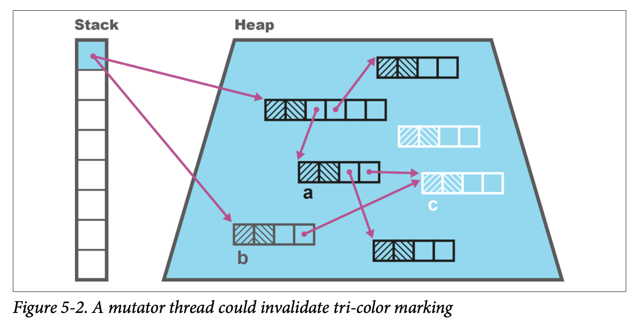
If all references from gray objects to the new white object are now deleted, we have a situation where the white object should still be reachable but will be deleted, as it will not be found, according to the rules of the algorithm.

This problem can be solved in a couple different ways. We could, for example, change the color of the black object back to gray, adding it back to the set of nodes that need processing as the mutator thread processes the update.

That approach, using a “write barrier” for the update, would have the nice algorithmic property that it would maintain the tri-color invariant throughout the whole of the marking cycle.

info

Tri-color invariant: no black object node may hold a reference to a white object node during concurrent marking.

However, this comes at a cost—it destroys a property (“monotonicity”) needed for a simple proof that the marking algorithm terminates.

An alternative approach is to keep a queue of all changes that could potentially violate the invariant, and then have a secondary “fixup” phase that runs after the main phase has finished. This fixup must, of necessity, be a STW phase, but in practice, it is usually very short.

The modern general purpose collector, G1, uses the second approach (known as a remark phase)—we will discuss this in more detail when we meet it in “G1”. First, let’s talk about other important techniques for concurrent garbage collection.

Forwarding Pointers

In this section, we’ll discuss the use of forwarding pointers. These are also known as Brooks pointers after their inventor, Rodney Brooks. This technique, in its simplest form, uses an additional word of memory per object to indicate whether the object has been relocated during a previous phase of garbage collection and to give the location of the new version of the object’s contents.

The resulting heap layout (as used by early versions of the Shenandoah collector, for example) for its object pointers ( oops) can be seen in Figure 5-3. Note that if the object has not been relocated, then the Brooks pointer simply points at the start of the object header.

info

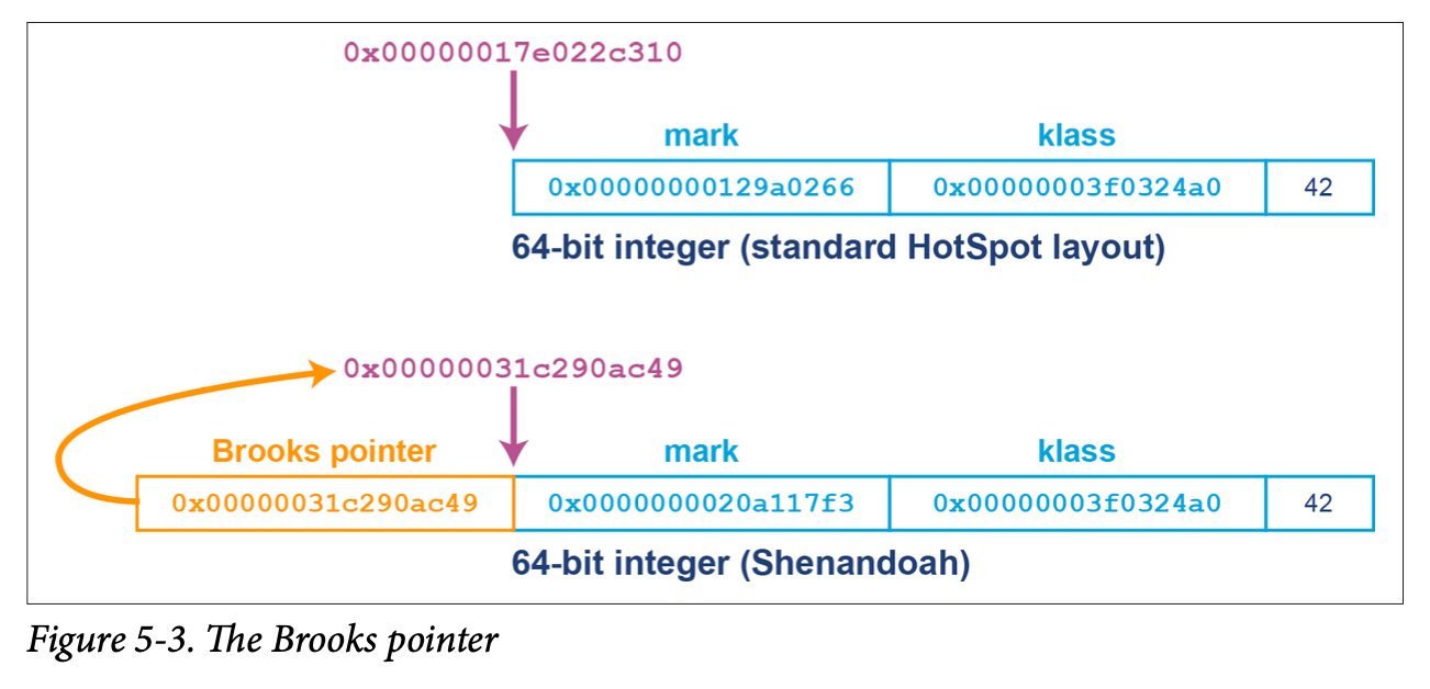
The Brooks pointer mechanism relies upon the availability of hardware compare-and-swap (CAS) operations to provide atomic updates of the forwarding address.

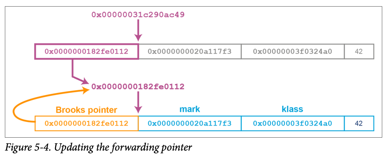
During a concurrent marking phase, the collector threads trace through the heap and mark any live objects. If an object reference points to an oop that has a forwarding pointer, then the reference is updated to point directly at the new oop location. This can be seen in Figure 5-4.

This can be a useful technique, but its obvious downside is that it requires an extra word of memory per object. For example, this increases the heap space required for an Integer object from 20 to 28 bytes. This can represent a significant additional overhead.

This technique is used by Shenandoah and other advanced collectors—we will have more to say about the practical usage of it later, including ways to mitigate the increased memory requirements. Let’s move on to meet our next major topic—the G1 collector that is the default for the HotSpot virtual machine for versions of Java newer than 8.

G1

G1 (the “Garbage First” collector) is a very different style of collector than the parallel collectors. It was first introduced in a highly experimental and unstable form in Java 6, but was extensively rewritten throughout the lifetime of Java 7, and it became stable and production-ready with the release of Java 8u40.

G1 was originally intended to be a replacement low-pause collector that superseded the Concurrent Mark Sweep (CMS) collector (which is no longer supported). It was designed to be a collector that was:

• Much easier to tune than CMS
• Less susceptible to premature promotion
• Capable of better scaling behavior (especially pause time) on big heaps
• Able to greatly reduce the need to fall back to full STW collections

However, over time, G1 evolved into being thought of as more of a general-purpose collector. It became the default collector in Java 9, taking over from the parallel collectors. G1 has continued to improve over subsequent Java releases—it is greatly improved in Java 11, and better still in Java 17 and 21.

One of the most important concepts in G1 is that of pause goals. These allow the developer to specify the desired maximum amount of time that the application should pause on each garbage collection cycle. Note that this is expressed as a goal, and there is no guarantee that the application will be able to meet it. If this value is set too low, then the GC subsystem will be unable to meet the goal.

The default value for pause goals is 200 ms—but in practice, pauses are usually much less than this, so the default value is usually fine for most applications with typical heap sizes. For applications with very large heaps (tens or hundreds of gigabytes), the pause goal may need to be adjusted.

info

Garbage collection is driven by allocation, which can be highly unpredictable for many Java applications. This can limit or destroy G1’s ability to meet pause goals.

Another major difference that the design of the G1 collector has is that it rethinks the notion of generations as we have met them so far. Specifically, unlike the parallel collectors, G1 does not have dedicated, contiguous memory spaces per generation, and instead introduces regions.

G1 Heap Layout and Regions

The G1 heap is based upon the concept of fixed-sized regions that make up a generation. These are areas that are by default 1 MB in size (but are larger on bigger heaps). The use of regions allows for noncontiguous generations and makes it possible to have a collector that does not need to collect all garbage on each run (incremental collection).

info

The overall G1 heap is still contiguous in memory—it’s just that the memory that makes up each generation no longer has to be.

The region-based layout of the G1 heap can be seen in Figure 5-5.

As you can see, G1 still has a concept of a young generation made up of Eden and survivor regions.

As of Java 21, G1’s algorithm allows regions of a power of 2 MB—so 1, 2, 4 ... MB, with the max size being 512 MB. By default, it expects between 2,048 and 4,095 regions in the heap and will adjust the region size to achieve this.

To calculate the region size, we compute this value:

<Heap size> / 2048

and then round it down to the nearest permitted region size value. Then the number of regions can be calculated:

Number of regions = <Heap size> / <region size>

As usual, we can change the value of the region size by applying a configuration option, but in practice this is rarely necessary.

If an application creates an object that occupies more space than half a region size, then it is considered a humongous object.

These objects are directly allocated in special humongous regions, which are free, contiguous regions that are immediately made part of the tenured generation (rather than Eden). The typical case for this is large arrays (as arrays are objects in Java).

G1 Collections

G1 has two kinds of collections:

Young GC (aka G1New) – The regions to be collected include only young regions.

Mixed GC (aka G1Old) – The collection set contains both young and old regions.

A young collection is a STW collection seeking to reclaim as much heap as fast as possible. It does so by completely evacuating regions so they can immediately be reused.

While warming up, the collector keeps track of the statistics of how many “typical” regions can be collected per GC run. If enough memory can be collected to balance the new objects that have been allocated since the last GC, then the collector is not losing ground to allocation, and G1New collections will continue. This means that pause times can be controlled, as long as the collector can stay ahead of the allocation rate.

A mixed collection is a mostly concurrent collection used when the number of old objects has risen sufficiently that a young collection is no longer sufficient to reclaim enough memory to balance allocation. At this point, it is worth expending extra effort to reclaim old objects and increase the number of free regions.

The point when a mixed collection will start is known as the Initiating Heap Occupancy Percent (IHOP) threshold. G1 automatically determines IHOP based on earlier application behavior. The default initial value is 45% (but this can be changed with a config switch), and the application will adjust up or down adaptively.

This gives us a reasonable high-level picture of the collector, i.e., that G1:

• Is a regional, generational collector
• Is an evacuating collector
• Provides “statistical compaction”
• Uses a concurrent marking phase (for mixed collections)

The concepts of TLAB allocation, evacuation to survivor space, and promoting to tenured are broadly similar to the other HotSpot GCs you’ve already met.

However, G1 mixed collections are a little more complex than the collections we’ve already discussed, so let’s take a closer look.

G1 Mixed Collections

One of the most often overlooked aspects of G1 is, bizarrely, its great strength. Specifically, G1 mixed collections mostly run concurrently with application threads. By default, some of the available cores (at least one) will perform the concurrent phases of G1, and the other half will continue to execute application code.

info

The exact formula for ConcGCThreads—the number of cores used for concurrent GC—is a little complicated:

max(1, (ParallelGCThreads + 2) / 4)

where ParallelGCThreads is usually the number of cores, at least on small machines.

This has two main consequences:

• Application throughput is reduced while a mixed collection is running.
• It is possible for the application to need to perform a young GC while a concur‐ rent collection is underway.

Note that in the case where a young GC needs to run during a mixed collection, it will typically take longer to complete than normal, as the young GC will have only a reduced number of cores to work with.

G1Old has four phases:

1. Concurrent Start (includes a STW G1New)
2. Concurrent Mark
3. Remark (STW)
4. Cleanup (STW)

The purpose of the Concurrent Start phase is to provide a stable set of starting points for GC that are within each region; these are the GC roots for the purposes of the collection cycle. After the initial marking has concluded, the Concurrent Mark phase commences. This essentially runs a form of the tri-color marking algorithm on the heap, keeping track of any changes that might later require fixup.

The Concurrent Mark phase typically takes much longer than the others. This means that for most of its run time, G1Old runs alongside application threads. However, for three phases (Concurrent Start, Remark, and Cleanup), all application threads must be stopped. The overall effect (as compared to ParallelOld) should be to replace a single long STW pause with three STW pauses, which are usually very short.

After the Concurrent Mark, G1Old must fix up its records to avoid violating the first rule of garbage collectors—collecting an object that is still alive. This is the Remark phase, and a substantial amount of work has been done to remove tasks from this STW phase and move them into the Concurrent Mark phase.7

The Cleanup phase is mostly STW and comprises accounting tasks that identify regions that are now completely free and ready to be reused (e.g., as Eden regions).

Remembered Sets

Recall that when we met the ParallelOld collector, the heuristic “few references from old to young objects” was discussed, in “Weak Generational Hypothesis” on page 86. HotSpot uses a mechanism called card tables to help take advantage of this phenomenon in the parallel (and also CMS) collectors.

The G1 collector has a related feature to help with region tracking. The Remembered Sets (usually just called RSets) are per-region entries that track outside references that point into a heap region.

This means that instead of tracing through the entire heap for references that point into a region, G1 just needs to examine the RSets and then scan those regions for references.

Figure 5-6 shows how the RSets are used to implement G1’s approach to dividing up the work of GC between allocator and collector.

RSets (and also card tables in Parallel) is a technique that can contribute to a GC problem called floating garbage. This is an issue caused when objects that are otherwise dead are kept alive by references from dead objects outside the current collection set. That is, on a global mark they can be seen to be dead, but a more limited local marking may incorrectly report them as alive, depending on the root set used. RSets could cause increased floating garbage due to scanning pointers from dead objects within the region.

During the Cleanup phase of a mixed collection, G1 performs RSet “scrubbing.” This is a process that looks at the RSets of regions that pointed into evacuated regions and updates references to objects that have been moved to other regions.

Full Collections

A full GC is an STW collection similar to the full collections we have already met in the parallel collectors.

A full GC cleans the entire heap—both young and tenured spaces (old gen). It also compacts the objects in the humongous regions in place—they are not included in normal evacuation phases to reduce copying overhead.

Full GCs can be caused in several ways—one of them is via fragmentation of the humongous regions. If this occurs, then allocation of humongous objects can fail, even though there is enough free memory to satisfy the allocation request ( because the free space is not in a contiguous block).

Another possibility is that if the Concurrent Mark phase during a mixed collection is not able to finish before the application has allocated all available heap memory, then G1 will have no choice but to perform a full GC—this is sometimes called a concurrent mode failure.

Normally, the IHOP threshold is set dynamically so that this does not happen; however, if the application’s allocation profile changes, the predicted value (based on past behavior) might be wrong.

To avoid this type of full GC, the obvious thing to do is to start a concurrent marking phase earlier—this will usually happen adaptively, but for some workloads, a different IHOP threshold may need to be set manually with a config switch.

JVM Config Flags for G1

If you’re still running Java 8, then the switch that you need to enable G1 is:

+XX:UseG1GC

For modern versions of Java, no switch is needed—but be careful when running in containers. If your container only has a single visible core, then G1 will not be able to run concurrently (as there is only core) and will fall back to the serial collector. This is unlikely to be what you want.

As we mentioned earlier, G1 is based around pause goals. The switch that controls this core behavior of the collector is:

-XX:MaxGCPauseMillis=200

In other words, the default pause time goal is 200 ms. In practice, if your heap size is single-digit numbers of gigabytes, then the collector will probably never get anywhere near this value—and your STW times will be a lot lower.

If concurrent mode failures are causing too-frequent full GCs, then it is possible to adjust the IHOP threshold. The first thing to try is to ask the JVM to reduce the threshold for when to start mixed collections. This is done by increasing the buffer size used in IHOP calculation:

-XX:G1ReservePercent=10

It is also possible to disable the adaptive calculation of IHOP by setting it manually, although this is not recommended for most applications and should be attempted only if the adaptive approach has been unsuccessful. This is done using a pair of switches:

-XX:-G1UseAdaptiveIHOP
-XX:InitiatingHeapOccupancyPercent=45

In some circumstances, you may want to keep the adaptive behavior, but just change the initial value of IHOP. In this case, you would only set

-XX:InitiatingHeapOccu pancyPercent=n.

One other option that may also be of use is the option of changing the region size, overriding the default algorithm:

-XX:G1HeapRegionSize=<n>m

Note that n must be a power of 2, between 1 and 512, as before, and must indicate a value in megabytes. The m suffix is mandatory, and if it is omitted, there may be unexpected results.

G1 has improved greatly since its introduction, and it is a superb general-purpose collector. However, it is not the only collector available for HotSpot—others exist, although they are usually suitable only for specific workloads.

Let’s move on to discuss Shenandoah, the first of these alternative collectors.

Shenandoah

An alternative to G1 is the Shenandoah collector. It was created by Red Hat within the OpenJDK project and was made available as an experimental collector in Java 12. It was productionized in Java 15, and is a fully supported collector in Java 17 and 21.8

Shenandoah’s goal is to bring down pause times on large (meaning tens or hundreds of gigabytes) heaps. There is no such thing as a free lunch, however, so Shenandoah potentially uses significantly more CPU resources than G1 to achieve this goal.

Shenandoah’s approach to achieving low latency on large heaps is to perform concurrent compaction. The resulting phases of collection in Shenandoah are:

1. Init Mark (STW)
2. Concurrent Mark
3. Final Mark (STW)
4. Concurrent Cleanup
5. Concurrent Evacuation
6. Init Update Refs (STW)
7. Concurrent Update Refs
8. Final Update Refs (STW)
9. Concurrent Cleanup

These phases may initially seem similar to those seen in G1, and some similar approaches (e.g., SATB) are used by Shenandoah. However, there are some fundamental differences.

Concurrent Evacuation

Let’s take a look at how the GC threads (which are running concurrently with app threads) perform evacuation. To make things a bit easier to understand, we’ll talk about the original version of Shenandoah, which was implemented using forwarding pointers:

1. Copy the object into a TLAB (speculatively).
2. Use a CAS operation to update the forwarding pointer to point at the speculative copy.
3. If this succeeds, then the compaction thread won the race, and all future accesses to this version of the object will be via the Brooks pointer.
4. If it fails, the compaction thread lost. It undoes the speculative copy and follows the Brooks pointer left by the winning thread.

As Shenandoah is a concurrent collector, while a collection cycle is running, more garbage is being created by the application threads. Therefore, collection has to be able to keep up with the production of new garbage; otherwise the application will suffer a concurrent mode failure.

JVM Config Flags for Shenandoah

Shenandoah can be activated with the following switch:

-XX:+UseShenandoahGC

A comparison of Shenandoah’s pause times as compared to other collectors can be seen in Figure 5-7.

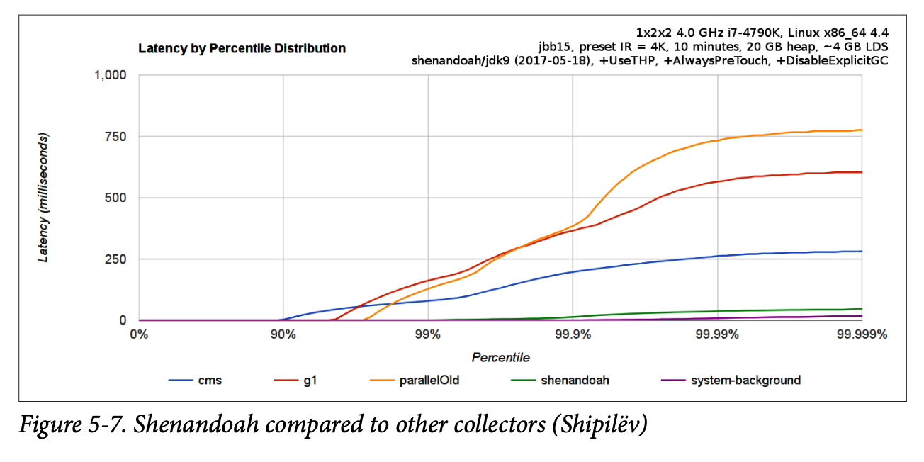
Compared to G1 and collectors such as Parallel, it is not anticipated that Shenandoah will require any special configuration by most users.

Shenandoah’s Evolution

Shenandoah’s design has evolved over time, and the current implementation is quite different from the original version. One area in which we see this is in the use of Brooks pointers. The original design of Shenandoah used the classical version of Brooks pointers, with the extra word of header at negative offset. However, it is possible to use a trick to avoid consuming the additional word of memory. To see how the trick works, notice that the use of a forwarding pointer has two aspects:

• It indicates that this version of the object may be invalid.
• It indicates the address at which the valid version of the object can be found.

It turns out to be possible to use a specific combination of bits in the mark word— a combination previously unused by HotSpot—to indicate that the object is invalid. In other words, we can directly indicate on the mark word that the object has been forwarded.

The contents of the rest of the storage for this object no longer matters—as the correct version of the object can be found by following the forwarding pointer. This means that some of the object’s memory can be used to store the forwarding pointer, so the extra word of memory in the object header is no longer needed. This trick could be implemented on the original version of Shenandoah, but it was not found to be an acceptable performance tradeoff at the time. However, this changed with the arrival of a technique known as loaded-reference barriers in HotSpot with Java 13. This opened the way for a new version of Shenandoah that shipped with Java 13 and contained these improvements.

Further improvements were made in subsequent releases, such as:

• Java 14: Self-fixing barriers
• Java 14: Concurrent class unloading
• Java 15: Concurrent reference processing
• Java 17: Concurrent thread-stack processing

The end result is that the Java 17 version of Shenandoah is production-ready, as are Red Hat’s backports. However, it’s worth being reminded that it is not considered a general-purpose collector—it is intended for use on large heaps only.

One other note of caution is that, at the time of writing, Shenandoah is not a generational collector. Attempts are under way to add this feature, but it is not yet available.

Let’s move on to meet the next alternative collector for HotSpot—ZGC.

ZGC

Oracle has also been working on a collector that serves a similar purpose to Shenandoah, known as ZGC. The intent is to deliver a collector in which all GC operations that scale with the size of the heap or the size of metaspace are moved out of safepoints (i.e., STW phases) and into concurrent phases.

The major user-visible goal for ZGC is to meet the user expectation that time spent inside of GC safepoints does not exceed one millisecond on heaps up to 1 TB (although ZGC can handle heap sizes up to 16 TB).

ZGC was first introduced as an experimental collector for Linux/x64 in Java 11 and has evolved significantly from that initial starting point. It is now a fully supported collector in Java 17 and 21, across a range of operating systems.

In theoretical terms, we can say that ZGC is:

• Concurrent
• Region-based
• Compacting
• Aware of non-uniform memory access (NUMA)
• Using colored pointers
• Using load barriers

This means that it is somewhat similar to G1 and Shenandoah in some aspects—for example, ZGC is a concurrent, region-based collector.

Not only this, but some of the key technologies and techniques (e.g., concurrent reference and thread-stack processing) that Shenandoah relies upon were initially implemented by the ZGC team and then utilized by both collectors. ZGC also uses a version of remembered sets (similar to G1).

However, in other respects, ZGC is quite different from the other collectors.

For example, one other important implementation detail is that ZGC does not use Brooks pointers but instead utilizes colored pointers.

This technique stores additional metadata about object lifecycle in the object pointer/oop itself. The metadata describes such things as whether the object is known to be alive and whether the address is correct (i.e., if this is the canonical copy of the object). This oop layout can be seen in Figure 5-8.

When a load barrier is encountered, the GC thread will check the colored pointer and ensure it is the expected value before proceeding.

info

For ZGC there are no compressed oops—so the colored pointer is always 64 bits. This provides for 44 bits of heap addressing, which is sufficient for heaps up to 16 TB in size.

Standard ZGC uses multimapping, so each physical page of memory is referred to by multiple virtual pages. This can lead to misleading numbers—the traditional RSS number can over-report heap usage when using ZGC by as much as 3x, compared to the accurate PSS figure.

ZGC can be enabled with this switch:

-XX:+UseZGC

It is a major goal of ZGC to avoid requiring users to tune the collector. For example, ZGC has no IHOP (in the sense of G1) but instead uses a cost model to decide when to start a collection. As another example, the number of threads used for GC is also a dynamic property of ZGC—including being able to change the size of the GC thread pool during a collection.

ZGC has been widely used for production workloads for several years now, but until now, there has always been a potential issue with it—it has not been a generational collector.

Java 21 introduced a new version of ZGC, known as Generational ZGC. Nongenerational ZGC is the older version of ZGC—and as you might expect from the name, it doesn’t take advantage of generations to optimize its runtime characteristics. Nongenerational collectors are more susceptible to allocation stalls, as they cannot perform a quick young GC to reclaim space. Adding generations to ZGC is, therefore, a useful step forward, as it helps to reduce the impact of a highly variable allocation rate.

Generational ZGC uses the terms minor and major for its collections—minor collections affect only the young objects, whereas major collections run over the entire heap. In this way, they are similar to the young and mixed collections of G1. As noted in the previous section, nongenerational ZGC uses multimapped memory, which can cause over-reporting of memory usage. Generational ZGC avoids this by using explicit code in the memory barriers instead. Generational ZGC also uses a different approach to colored pointers--it uses 12 color bits instead of 4, as you can see in Figure 5-9.

We should also note that the references stored on the JVM stack are implemented as colorless pointers, and the GC algorithm needs to translate these into colored pointers before they can be used in the heap.

This is a significant increase in complexity over the version used by nongenerational ZGC; however, it does open the door to some interesting optimizations, and the long-term intent is for Generational ZGC to completely replace the nongenerational version.

info

More detail of how Generational ZGC is implemented can be found in JEP 439.

Generational ZGC is enabled with these command-line options:

-XX:+UseZGC -XX:+ZGenerational

Current users of the older version are encouraged to transition to use the newer Generational version of ZGC.

Let’s move on to meet the final collector that we will discuss in this chapter—the Balanced collector of the OpenJ9 JVM.

Balanced (Eclipse OpenJ9)

The Eclipse open source foundation maintains a JVM called OpenJ9. This was historically a proprietary JVM produced by IBM, but it was made open source several years ago. The VM has several different collectors that can be switched on, including a high-throughput collector similar to the parallel collector HotSpot defaults to.

In this section, however, we will discuss the Balanced collector. It is a region-based collector available on 64-bit JVMs and designed for heaps in excess of 4 GB. Its primary design goals are to:

• Improve scaling of pause times on large Java heaps.
• Minimize worst-case pause times.
• Utilize awareness of NUMA performance.

To achieve the first goal, the heap is split into a number of regions, which are man‐ aged and collected independently. Like G1, the Balanced collector wants to manage at most 2,048 regions, so it will choose a region size to achieve this. The region size is a power of 2, as for G1, but Balanced will permit regions as small as 512 KB.

As we would expect from a generational region-based collector, each region has an associated age, with age-zero regions (Eden) used for allocation of new objects. When the Eden space is full, a collection must be performed. The IBM term for this is a partial garbage collection (PGC).

A PGC is an STW operation that collects all Eden regions and may additionally choose to collect regions with a higher age, if the collector determines that they are worth collecting. In this manner, PGCs are similar to G1’s mixed collections.

info

Once a PGC is complete, the age of regions containing the surviv‐ ing objects is increased by 1. These are sometimes referred to as generational regions.

Another benefit, as compared to other OpenJ9 GC policies, is that class unloading can be performed incrementally. Balanced can collect class loaders that are part of the current collection set during a PGC. This is in contrast to other OpenJ9 collectors, where class loaders could be collected only during a global collection.

One downside is that because a PGC only has visibility of the regions it has chosen to collect, this type of collection can suffer from floating garbage. To resolve this problem, Balanced employs a global mark phase (GMP). This is a partially concurrent operation that scans the entire Java heap, marking dead objects for collection. Once a GMP completes, the following PGC acts on this data. Thus, the amount of floating garbage in the heap is bounded by the number of objects that died since the last GMP started.

The final type of GC operation that Balanced carried out is global garbage collection (GGC). This is a full STW collection that compacts the heap. It is similar to the full collections that would be triggered in HotSpot by a concurrent mode failure.

OpenJ9 Object Headers

The basic OpenJ9 object header is a class slot, the size of which is 64 bits, or 32 bits when compressed references is enabled.

Compressed references is the default for heaps smaller than 57 GB and is similar to HotSpot’s compressed oops technique.

However, the header may have additional slots, depending on the type of object:

• Synchronized objects will have monitor slots.
• Objects put into internal JVM structures will have hashed slots.

In addition, the monitor and hashed slots are not necessarily adjacent to the object header—they may be stored anywhere in the object, taking advantage of otherwise wasted space due to alignment. OpenJ9’s object layout can be seen in Figure 5-10.

The highest 24 (or 56) bits of the class slot are a pointer to the class structure, which is off-heap, similarly to Java’s Metaspace. The lower 8 bits are flags that are used for various purposes depending on the GC policy in use.

Large Arrays in Balanced

Allocating large arrays in Java is a common trigger for compacting collections, as enough contiguous space must be found to satisfy the allocation. We saw one aspect of this in the discussion of G1, where humongous object allocation results in frag‐ mentation and insufficient space for a large allocation—resulting in a concurrent mode failure.

For a region-based collector, it is entirely possible to allocate an array object in Java that exceeds the size of a single region. To address this, Balanced uses an alternate representation for large arrays that allows them to be allocated in discontiguous chunks. This representation is known as arraylets, and this is the only circumstance under which heap objects can span regions.

The arraylet representation is invisible to user Java code, and instead is handled transparently by the JVM. The allocator will represent a large array as a central object, called the spine, and a set of array leaves. The leaves contain the actual entries of the array and are pointed to by entries of the spine. This enables entries to be read with only the additional overhead of a single indirection. An example can be seen in Figure 5-11.

info

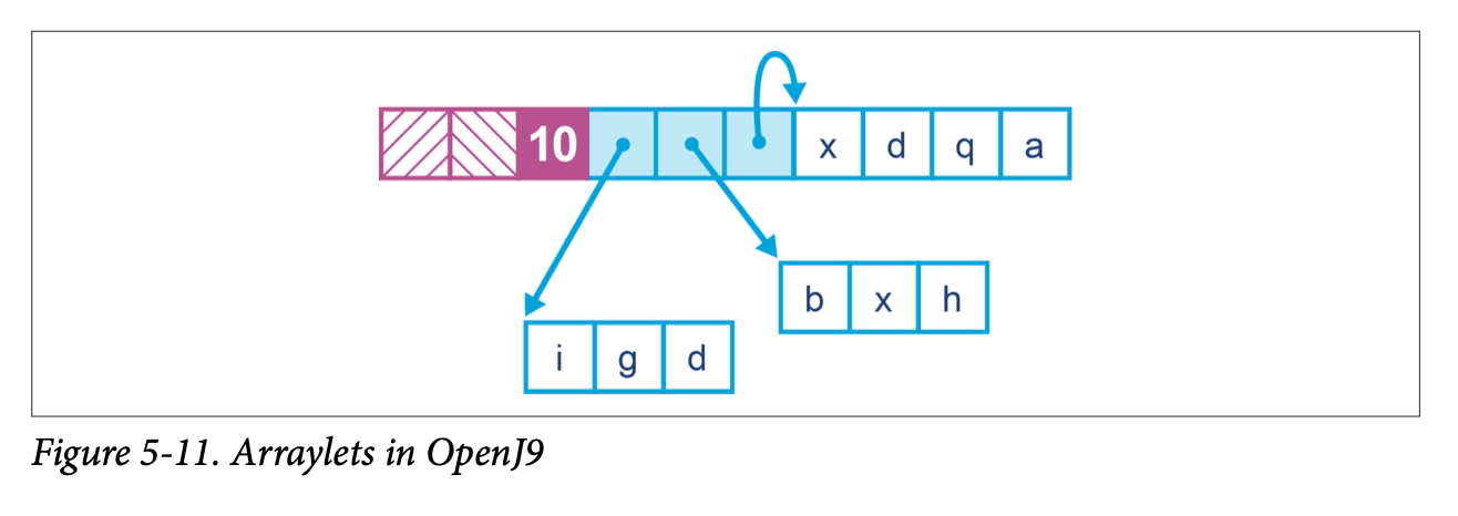
The arraylet representation is potentially visible through JNI APIs (although not from regular Java), so the programmer should be aware that when porting JNI code from another JVM, the spine and leaf representation may need to be taken into account.

Performing partial GCs on regions reduces average pause time, although overall time spent performing GC operations may be higher due to the overhead of maintaining information about the regions of a spine and its leaves. Crucially, the likelihood of requiring a global STW collection or compaction (the worst case for pause times) is greatly reduced, with this typically occurring as a last resort when the heap is full.

There is an overhead to managing regions and discontiguous large arrays, and thus, Balanced is suited to applications where avoiding large pauses is more important than outright throughput.

NUMA and Balanced

Non-uniform memory access is a memory architecture used in multiprocessor systems, typically medium to large servers. Such a system involves a concept of distance between memory and a processor, with processors and memory arranged into nodes. A processor on a given node may access memory from any node, but access time is significantly faster for local memory (that is, memory belonging to the same node).

For JVMs that are executing across multiple NUMA nodes, the Balanced collector can split the Java heap across them. Application threads are arranged such that they favor execution on a particular node, and object allocations favor regions in memory local to that node. A schematic view of this arrangement can be seen in Figure 5-12.

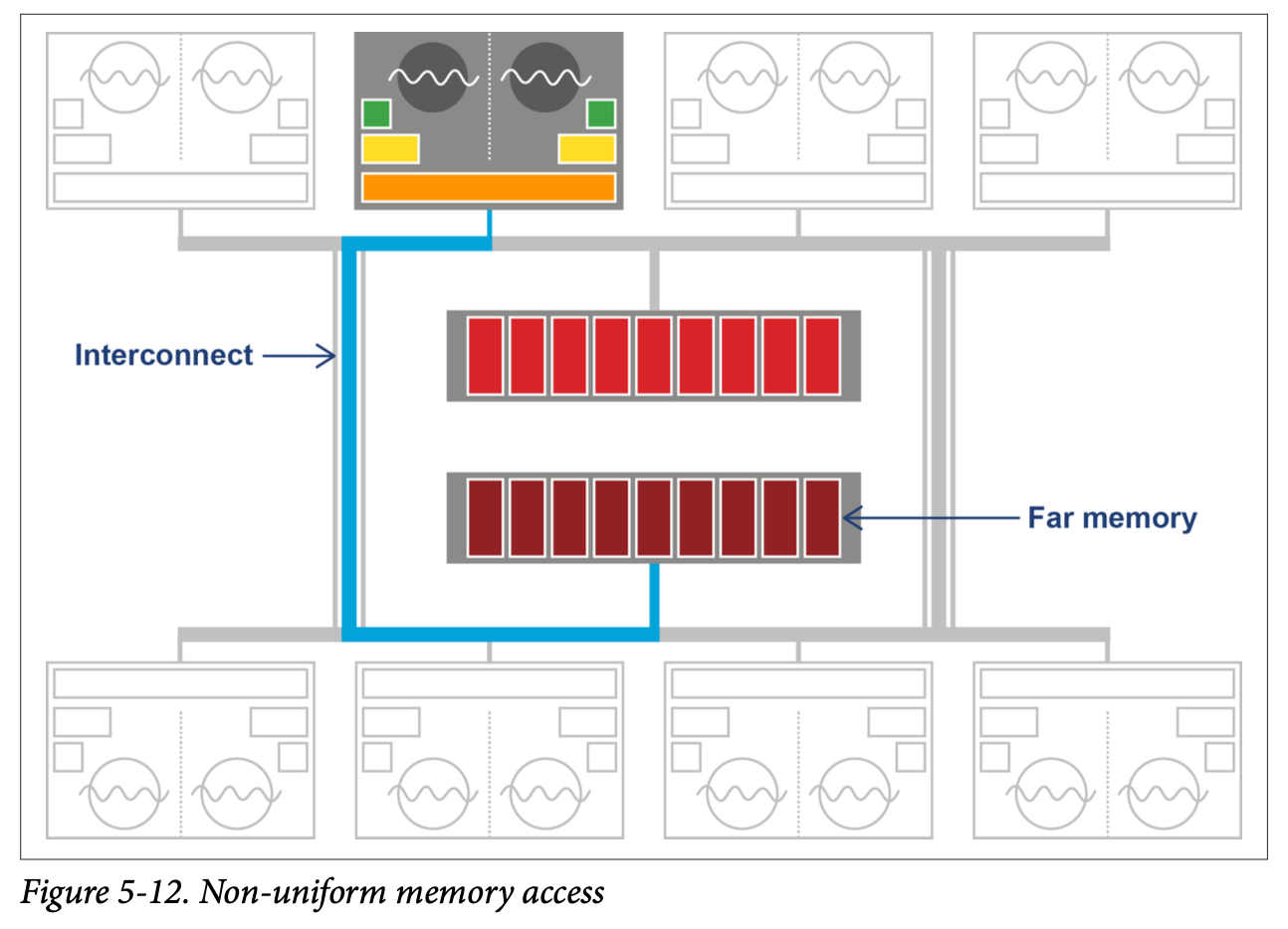
In addition, a partial garbage collection will attempt to move objects closer (in terms of memory distance) to the objects and threads that refer to them. This means the memory referenced by a thread is more likely to be local, improving performance. This process is invisible to the application.

Niche HotSpot Collectors

In earlier versions of HotSpot, various other collectors were available. Most of them have been removed, but as of Java 21, two niche collectors still exist. We mention them for completeness here, but neither is recommended for production use.

CMS

The Concurrent Mark Sweep (CMS) collector was designed to be an extremely low-pause collector for the tenured (aka old generation) space only. It was paired with a slightly modified parallel collector for collecting the young generation—called ParNew rather than Parallel GC.

It is present in Java 8 and 11, but it was deprecated in Java 9, and is no longer available as of Java 14.12 In practice, for Java 8, CMS still outperforms G1 for certain workloads that require a low-pause GC. However, G1 improved very significantly between Java 8 and 11. As a result, the workloads for which CMS is the best choice are much rarer for Java 11—and, of course, the collector is not available at all for Java 17 or 21.

The CMS collector is activated with the following flag:

-XX:+UseConcMarkSweepGC

CMS has a broadly similar phase structure to a G1 mixed collection in terms of its GC duty cycles. So, an important question is: what happens if Eden fills up while CMS is running?

The answer is, unsurprisingly, that because application threads cannot continue, they pause, and a (STW) young GC runs while CMS is running. This young GC run will usually take longer than in the case of the parallel collectors, because it has only half the cores available for young generation GC (the other half of the cores are running CMS).

Under normal circumstances, the young collection promotes only a small number of objects to tenured, and the CMS old collection completes normally, freeing up space in tenured. The application then returns to normal processing, with all cores released for application threads.

However, consider the case of a very high allocation rate, perhaps with premature promotion. This can potentially cause a situation in which the young collection has too many objects to promote for the available space in tenured. This is a form of concurrent mode failure, and the JVM has no choice at this point but to fall back to a collection using ParallelOld, which is fully STW. Effectively, the allocation pressure was so high that CMS did not have time to finish processing the old generation before all the “headroom” space to accommodate newly promoted objects filled up.

To avoid frequent concurrent mode failures, CMS needs to start a collection cycle before tenured is completely full. This is similar to the IHOP behavior of G1 that we met in “Concurrent Evacuation” on page 123.

Epsilon

The Epsilon collector is not a legacy collector. However, it is included here because it must not be used in production under any circumstances. While CMS, if encountered within your environment, should be flagged as high risk and marked for immediate analysis and removal, Epsilon is slightly different.

Epsilon is an experimental collector designed for testing purposes only. It is a zero- effort collector. This means it makes no effort to actually collect any garbage. Every byte of heap memory that is allocated while running under Epsilon is effectively a memory leak. It cannot be reclaimed and will eventually cause the JVM (probably very quickly) to run out of memory and crash.

info

Develop a GC that only handles memory allocation, but does not implement any actual memory reclamation mechanism. Once available Java heap is exhausted, perform the orderly JVM shutdown. —JEP 318: Epsilon: A No-Op Garbage Collector

Such a “collector” can be useful for the following purposes:

• Performance testing and microbenchmarks
• Regression testing
• Testing low/zero-allocation Java application or library code

In particular, Java Microbenchmark Harness (JMH tests would benefit from the ability to confidently exclude any GC events from disrupting performance numbers. Memory allocation regression tests, ensuring that changed code does not greatly alter allocation behavior, would also become easy to do. Developers could write tests that run with an Epsilon configuration that accepts only a bounded number of allocations and then fails on any further allocation due to heap exhaustion.

Finally, the proposed VM-GC interface would also benefit from having Epsilon as a minimal test case for the interface itself.

Summary

Garbage collection is a truly fundamental aspect of Java performance analysis and tuning. Java’s rich landscape of garbage collectors is a great strength of the platform, but it can be intimidating for the newcomer, especially given the scarcity of docu‐ mentation that considers the tradeoffs and performance consequences of each choice.

In this chapter, we have outlined the decisions that face performance engineers and the tradeoffs they must make when deciding on an appropriate collector to use for their applications. We have discussed some of the underlying theory and met a range of modern GC algorithms that implement these ideas.

In the next chapter, we will put some of this theory to work and introduce logging, monitoring, and tooling as a way to bring some scientific rigor to our discussion of performance-tuning garbage collection.