4. Understanding Garbage Collection

In this chapter, we will be introducing the garbage collection subsystems of the JVM. We will approach this by starting with an overview of the basic theory of mark and sweep (also known as tracing garbage collection). Then, we’ll look at the low-level features of the HotSpot runtime and how it represents Java objects at runtime.

In the second half of the chapter, we’ll talk about the key concepts of allocation and lifetime before discussing two key techniques that HotSpot uses to help with allocation. Then we’ll bring together all the topics we’ve met and introduce the simplest of HotSpot’s production collectors, the parallel collectors, and explain some of the details that make them useful for many production workloads.

Let’s begin by noting that the Java environment has several iconic or defining features, and garbage collection is one of the most immediately recognizable.

The essence of Java’s garbage collection is that rather than requiring the programmer to understand the precise lifetime of every object in the system, the runtime should keep track of objects on the programmer’s behalf and automatically get rid of objects that are no longer required. The automatically reclaimed memory can then be wiped and reused. However, when the platform was first released, there was considerable hostility to GC. This was fueled by the fact that Java deliberately provided no language-level way to control the behavior of the collector (and continues not to, even in modern versions).

This meant that, in the early days, there was a certain amount of frustration over Java’s functionality—compounded by the not-great performance of Java’s GC. This fed into perceptions of the platform as a whole, and even today, you may encounter people who still assume, incorrectly, that Java GC is a problem. The truth is that, these days, Java’s GC is incredibly fast (best in class) and entirely suitable for the vast majority of production workloads.

In fact, the early vision of mandatory, non-user-controllable GC has been more than vindicated, and these days very few application developers would attempt to defend the opinion that memory should be managed by hand. Even modern takes on systems programming languages (e.g., Rust and Go) regard memory management as the proper domain of the compiler and runtime, respectively, rather than the programmer.

There are two basic rules of garbage collection that all implementations strive to adhere to:

• No live object must ever be collected.
• Algorithms must collect all garbage.

Of these two rules, the first is by far the more important. Collecting a live object could lead to segmentation faults or (even worse) silent corruption of program data. Java’s GC algorithms need to be sure that they will never collect an object the program is still using.

If a GC algorithm consistently fails to collect some garbage, then the worst case is that, over time, the application will run out of memory and eventually crash. This is a terrible outcome, but even this is better than the alternative of collecting live objects and causing memory corruption.

However, having said this, the second rule has quite a lot of flexibility.

For example, the generational algorithms we will meet later in this chapter often leave older objects in the heap for a long time, until a full GC cycle is triggered. In addition, in the next chapter, we will meet algorithms that avoid collecting areas of memory that have not yet accumulated enough garbage.

Overall, the idea of the programmer surrendering some low-level control in exchange for not having to account for every low-level detail by hand is the essence of Java’s managed approach and expresses James Gosling’s conception of Java as a blue-collar language for getting things done.

Introducing Mark and Sweep

Most Java programmers, if pressed, can recall that Java’s GC relies on an algorithm called mark and sweep, but most also struggle to recall any details as to how the process actually operates.

In this section we will introduce a basic form of the algorithm and show how it can be used to reclaim heap memory automatically. This is deliberately simplified and is only intended to introduce a few basic concepts—it is not representative of how production JVMs actually carry out GC (we’ll meet those later).

This introductory form of the mark-and-sweep algorithm uses an allocated object list to hold a pointer to each object that has been allocated but not yet reclaimed. The overall GC algorithm can then be expressed as:

1. Loop through the allocated list, clearing the mark bit.
2. Starting from any pointers into the heap, find all the objects you can.
3. Set a mark bit on each object reached.
4. Loop through the allocated list, and for each object whose mark bit hasn’t been set:
   • Reclaim the memory in the heap and place it back on the free list.
   • Remove the object from the allocated list.

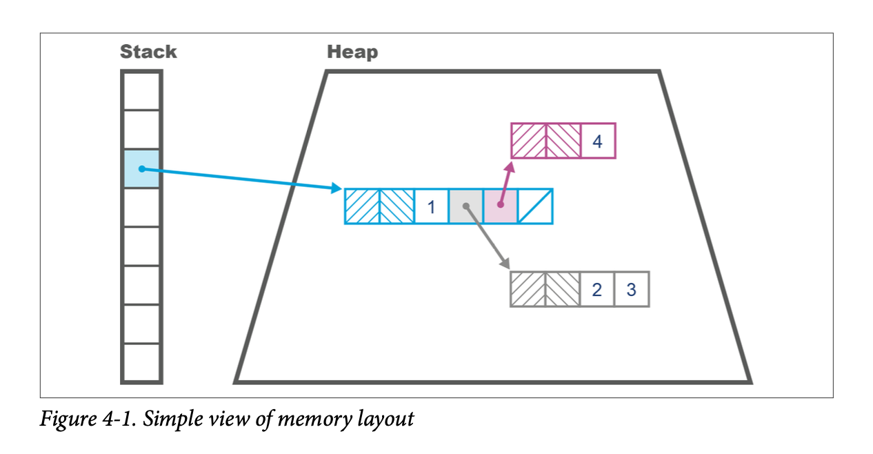
The live objects are usually located depth-first, and the resulting graph of objects is called the live object graph. It is sometimes also called the transitive closure of reachable objects, and an example can be seen in Figure 4-1. Conversely, unreachable objects are sometimes referred to as dead.

The state of the heap can be hard to visualize, but fortunately there are some simple tools to help us. One of the simplest is the jmap -histo command-line tool. This shows the number of bytes allocated per type, and the number of instances that are collectively responsible for that memory usage. It produces output like the following:

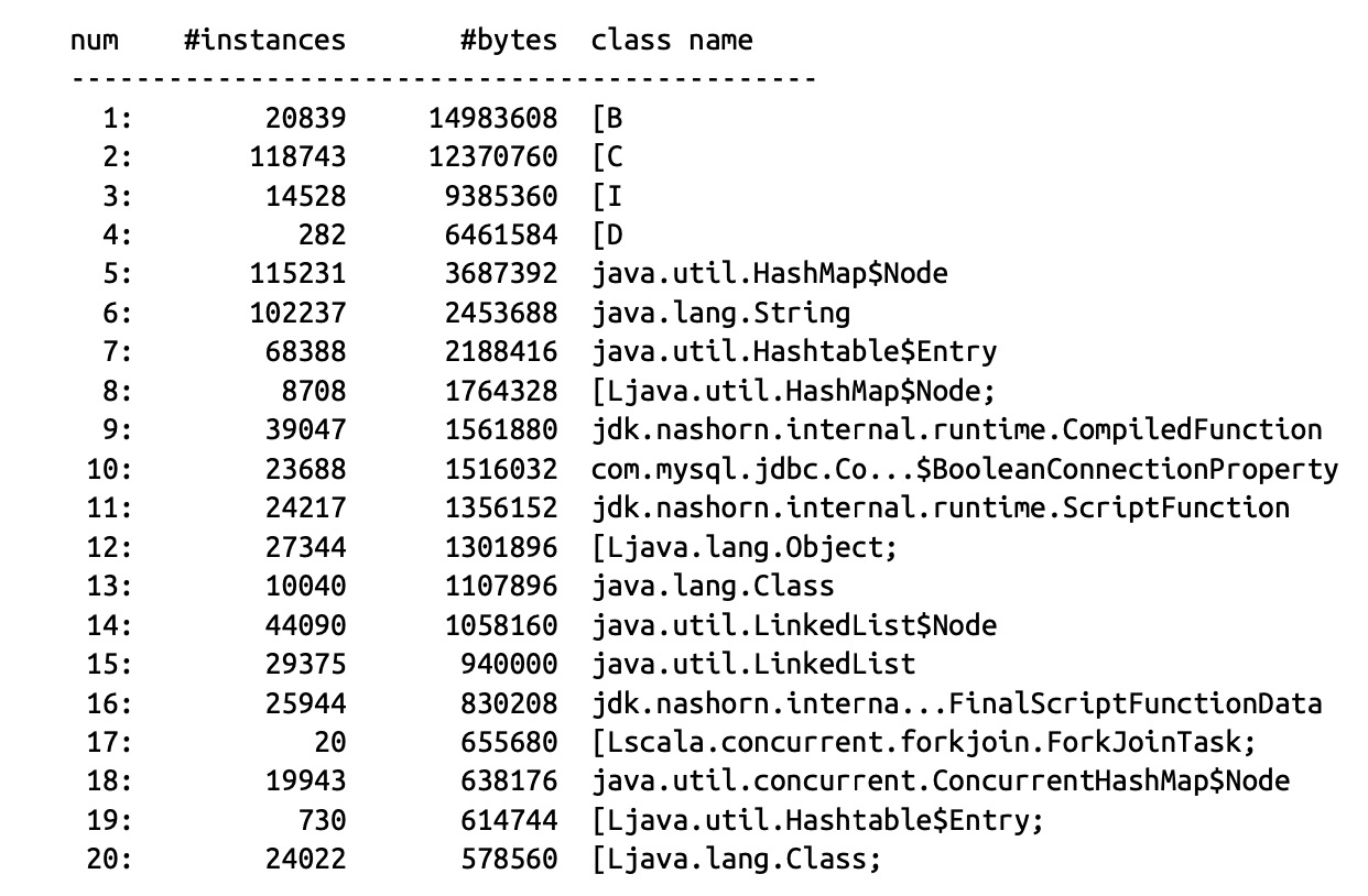
This shows a snapshot of the heap (and there are other, more complex and powerful tools such as Eclipse MAT available), but we may want to carry out live analysis instead.

In this case, we can use GUI tools such as the Sampling tab of VisualVM (introduced in Chapter 3) or the VisualGC plug-in to VisualVM. These tools provide a real-time view, which can be useful for a quick sense of how the heap is changing.

However, in general, the moment-to-moment view of the heap is not sufficient for accurate analysis. Instead, we should use a tool like JDK Flight Recorder (JFR) or GC logs for better insight into questions such as, “How big is my heap? How is it changing? Do I have a leak?"

Garbage Collection Glossary

The jargon used to describe GC algorithms is sometimes a bit confusing (and the meaning of some of the terms has changed over time). For the sake of clarity, we include a basic glossary of how we use specific terms:

Stop-the-world (STW) The GC cycle requires all application threads to be paused while garbage is collected. This prevents application code from invalidating the GC thread’s view of the state of the heap. This is the usual case for simple GC algorithms.

Concurrent GC threads can run while application threads are running. This is more difficult to achieve, and more expensive in terms of computation expended. HotSpot’s default collector (since Java 9) is Garbage First (G1), and it has some concurrent aspects, as we will see.

Parallel Multiple threads (and multiple cores) are used to execute garbage collection.

Exact An exact GC scheme has enough type information about the state of the heap to ensure that all garbage can be collected on a single cycle. More loosely, an exact scheme has the property that it can always tell the difference between a field that is an int and one that’s an object reference.

Conservative A conservative scheme lacks the information of an exact scheme. As a result, conservative schemes frequently fritter away resources and are typically far less efficient due to their fundamental ignorance of the type system they purport to represent.

Moving In a moving collector, objects can be relocated in memory. This means that they do not have stable addresses. Environments that (unlike Java) provide direct access to raw pointers are not a natural fit for moving collectors.

Compacting At the end of the collection cycle, allocated memory (i.e., surviving objects) is arranged as a single contiguous region (usually at the start of the region), and a pointer indicates the start of empty space that is available for objects to be written into. A compacting collector will avoid memory fragmentation.

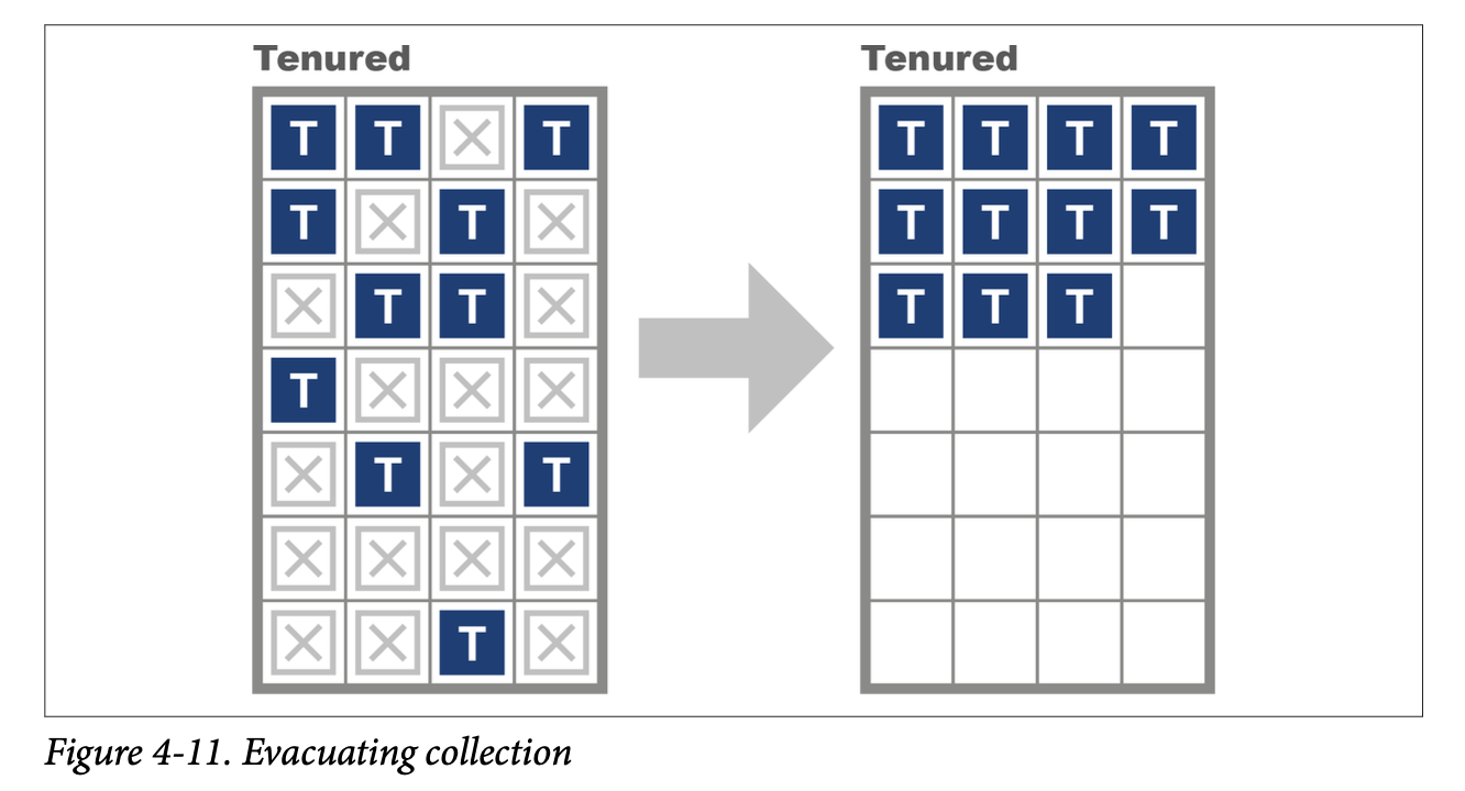
Evacuating At the end of the collection cycle, the collected region is totally empty, and all live objects have been moved (evacuated) to another region of memory. A good evacuating collector will avoid memory fragmentation.

In most other languages and environments, the same terms are used—but be careful, as some environments do things such as transpose the meaning of “concurrent” and “parallel,” or refer to “moving” as “copying.”

The term “concurrent” is also best understood as being a sliding scale rather than a binary state. Depending on the collector in use, more or less of the work of a collection can be performed concurrently with application threads.

Introducing the HotSpot Runtime

In addition to the general GC terminology, HotSpot introduces terms that are more specific to the implementation. To obtain a full understanding of how garbage collection works on this JVM, we need to get a grip on some of the details of HotSpot’s internals.

For what follows, it will be very helpful to remember that Java has only two sorts of value:

• Primitive types (byte, int, etc.)
• Object references

Many Java programmers loosely talk about objects, but for our purposes it is important to remember that, unlike C++, Java has no general address dereference mechanism and can only use an offset operator (the . operator) to access fields and call methods on object references.

Also, keep in mind that Java’s method call semantics are purely call-by-value, although for object references, this means that the value copied is the address of the object in the heap.

Representing Objects at Runtime

HotSpot represents Java objects at runtime via a structure called an oop. This is short for ordinary object pointer, and it is a genuine pointer in the C sense. These pointers can be placed in local variables of reference type, where they point from the stack frame of the Java method into the memory area comprising the Java heap.

One important fact to remember is that HotSpot does not use system calls to manage the Java heap. As we will see in Chapter 5, HotSpot manages the heap size from user space code, so we can use simple observables to determine whether the GC subsystem is causing some types of performance problems.

There are several different data structures that comprise the family of oops, and the sort that represent instances of a Java class are called instanceOops, or arrayOops if they represent an array. The general rule is that anything in the Java heap must have an object header.

Accordingly, the memory layout of an instanceOop starts with two machine words of header present on every object ( arrayOops have these, and an additional 32 bits of header—the array’s length). The mark word is the first of these and is a pointer that points at instance-specific metadata. Next is the klass word, which points at class-wide metadata. The klass word is used to locate the klass metatdata (or klass), which is held outside of the main part of the Java heap (but not outside the C heap of the JVM process). As they exist outside the Java heap, the klasses do not require an object header.

In Figure 4-2, we can see the difference for a simple case—on the top left an Entry object similar to the Map.Entry that we might use in a HashMap, and on the top right, the Entry.class object (e.g., obtained via getClass()). Both of these Java objects have klasses, which are shown below the dotted line:

record Entry<K, V>(int hash, K key, V value, Entry<K, V> next) {
}

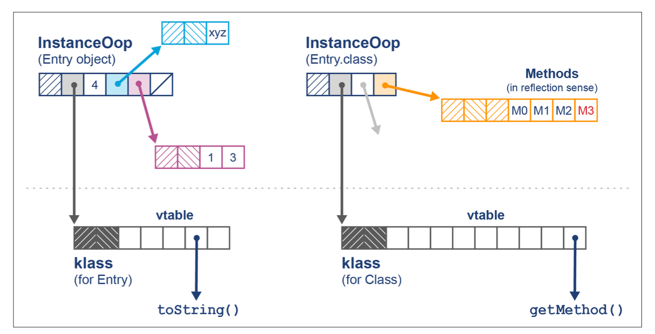
Fundamentally, the klass contains the virtual function table (or vtable) for the class, whereas the Class object contains (among other things) an array of references to Method objects for use in reflective invocation. We will have more to say on this subject in Chapter 6, when we discuss JIT compilation.

Oops are usually machine words, so 32 bits on a legacy 32-bit machine, and 64 bits on a modern processor. However, this has the potential to waste a possibly significant amount of memory. To help mitigate this, HotSpot provides a technique called compressed oops. If the option: -XX:+UseCompressedOops is set (and it is the default for 64-bit heaps), then the following oops in the heap will be compressed:

• The klass word of every object in the heap
• Instance fields of reference type
• Every element of an array of objects

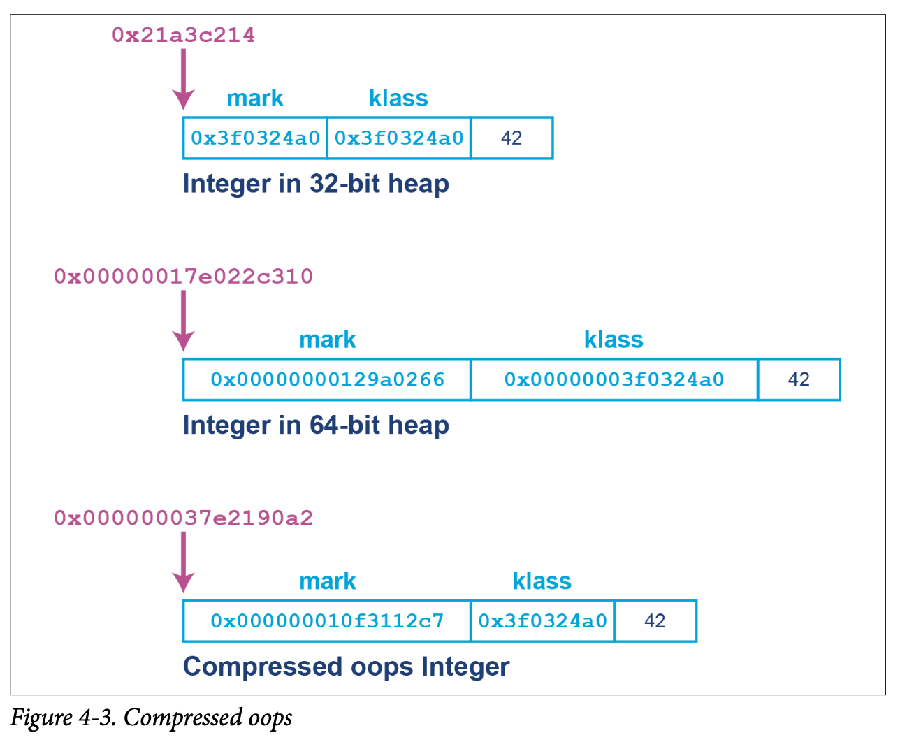
This means that, in general, a HotSpot object header consists of:

• Mark word at full native size
• Klass word (possibly compressed)
• 32 bits indicating the length if the object is an array
• A 32-bit gap (if required by alignment rules)

The instance fields of the object then follow immediately after the header. The memory layout for compressed oops can be seen in Figure 4-3.

In the past, some extremely latency-sensitive applications could occasionally see improvements by switching off the compressed oops feature—at the cost of increased heap size (typically an increase of 10%–50%). However, the class of applications for which this would yield measurable performance benefits is very small. For most modern applications, this would be a classic example of the antipattern known as Fiddling with Switches (see Appendix B for a full description).

As we remember from basic Java, arrays are objects. This means that the JVM’s arrays are represented as oops as well. This is why arrays have a third word of metadata as well as the usual mark and klass words—the array’s length. This also explains why array indices in Java are limited to 32-bit values, as the first versions of Java were purely for 32-bit architectures.

The managed environment of the JVM does not allow a Java reference to point anywhere but at an oop (or null). This means that at a low level:

• A Java value is a bit pattern corresponding either to a primitive value or to the address of an oop (a Java reference).
• Any Java reference considered as a pointer refers to the start of an object in the main part of the Java heap.
• Addresses that are the targets of Java references contain a mark word followed by a klass word as the next machine word.
• A klass and an instance of Class<?> are different (as the former lives in the metadata area of the heap), and a klass cannot be placed into a Java variable.

HotSpot defines a hierarchy of oops in .hpp files that are kept in src/hotspot/ share/oops in the main branch OpenJDK source tree.

The basic overall inheritance hierarchy for oops looks like this (as of Java 22):

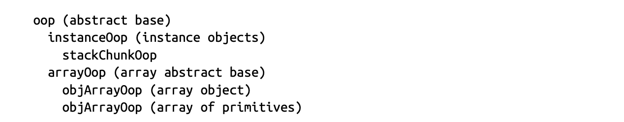
This use of oop structures to represent objects at runtime, with one pointer to house class-level metadata and another to house instance metadata, is not peculiar to Hot‐ Spot—many other JVMs and other execution environments use a related mechanism.

GC Roots

Articles and blog posts about HotSpot frequently refer to GC roots. These are “anchor points” for memory, essentially known pointers that originate from outside a memory pool of interest and point into it. They are external pointers as opposed to internal pointers, which originate inside the memory pool and point to another memory location within the memory pool.

We saw an example of a GC root in Figure 4-1. However, as we will see, there are other sorts of GC root, including:

• Stack frames
• Java Native Interface (JNI)
• Registers
• Code roots (from the JVM code cache)
• Globals
• Class metadata from loaded classes

If this definition seems rather complex, then the simplest example of a GC root is a local variable of reference type that will always point to an object in the heap (provided it is not null).

In the next section, we’ll take a closer look at two of the most important characteristics that drive the garbage collection behavior of any Java or JVM workload. A good understanding of these characteristics is essential for any developer who wants to really grasp the factors that drive Java GC (which is one of the key overall drivers for Java performance).

Allocation and Lifetime

The two primary drivers of the garbage collection behavior of a Java application are:

• Allocation rate
• Object lifetime

The allocation rate is the amount of memory used by newly created objects over some time period (usually measured in MB/s). This is not exposed by the JVM directly by default but is a relatively easy observable to estimate, and tools such as JFR can provide it (although there are potential performance implications for doing so, as we will discuss later in the book).

By contrast, the object lifetime is normally a lot harder to measure (or even estimate). In fact, one of the major arguments against using manual memory management is the complexity involved in truly understanding object lifetimes for a real application. As a result, object lifetime is, if anything, even more fundamental than allocation rate.

The idea that objects are created, they exist for a time, and then the memory used to store their state can be reclaimed is essential; without it, garbage collection would not work at all. As we will see in Chapter 5, there are a number of different tradeoffs that garbage collectors must balance—and some of the most important of these tradeoffs are driven by lifetime and allocation concerns.

Weak Generational Hypothesis

One key part of the JVM’s memory management relies upon an observed runtime effect of software systems, the weak generational hypothesis (WGH):

info

The distribution of object lifetimes on the JVM and similar software systems is bimodal—with the vast majority of objects being very short-lived and a secondary population having a much longer life expectancy.

This can be seen graphically in Figure 4-4.

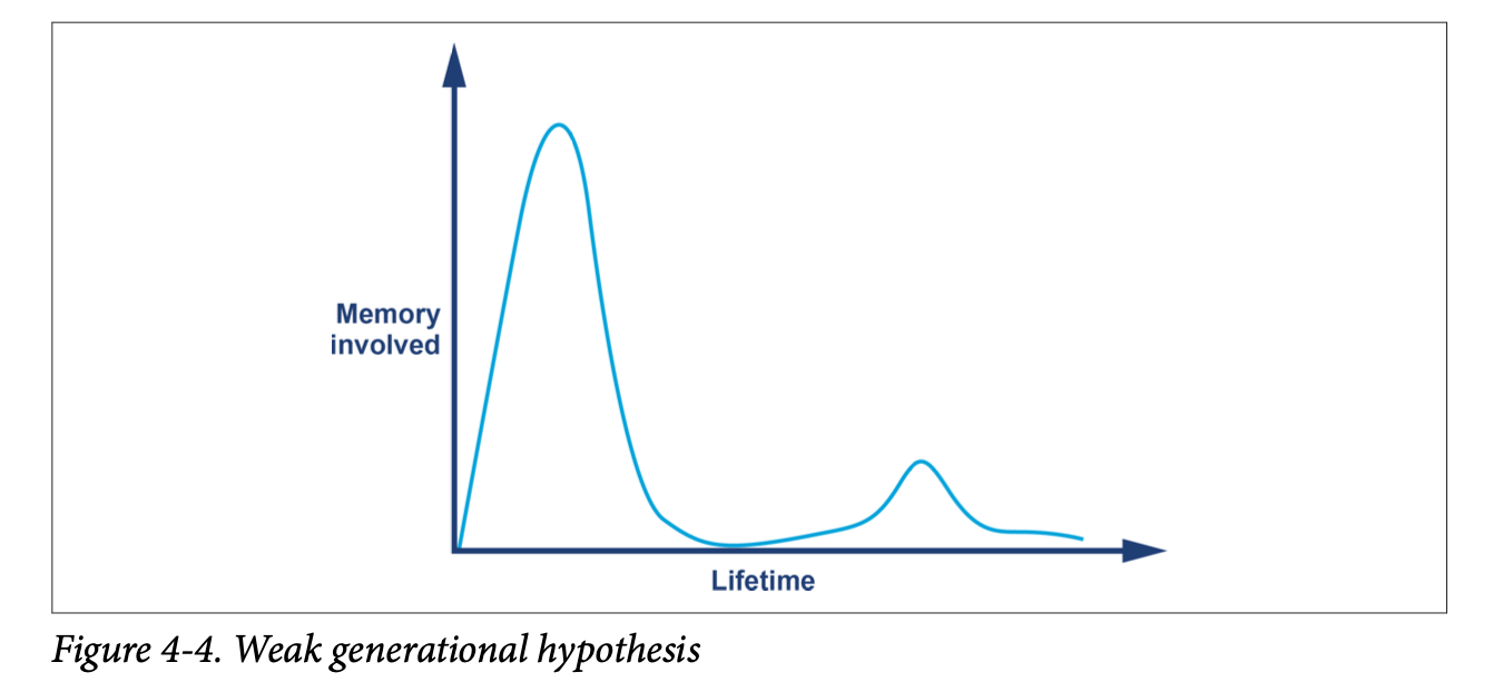
This hypothesis, which is really an experimentally observed and validated rule about the behavior of object-oriented workloads, leads to an obvious conclusion. That is, garbage-collected heaps should be structured in such a way as to allow short-lived objects to be easily and quickly collected, and for long-lived objects to be separated from short-lived objects.

This implies that the heap should have two separate areas—a short-lived area and a long-lived area—and that they should be collected separately in young and full collections, respectively.

One key technique is to use a mark-and-sweep collection on the recently created objects area—which is usually called Eden. During sweeping, the collector uses an evacuation phase to move any surviving objects to the long-lived space. Then the entire Eden space can be reclaimed at once.

We can see an image of this in Figure 4-5.

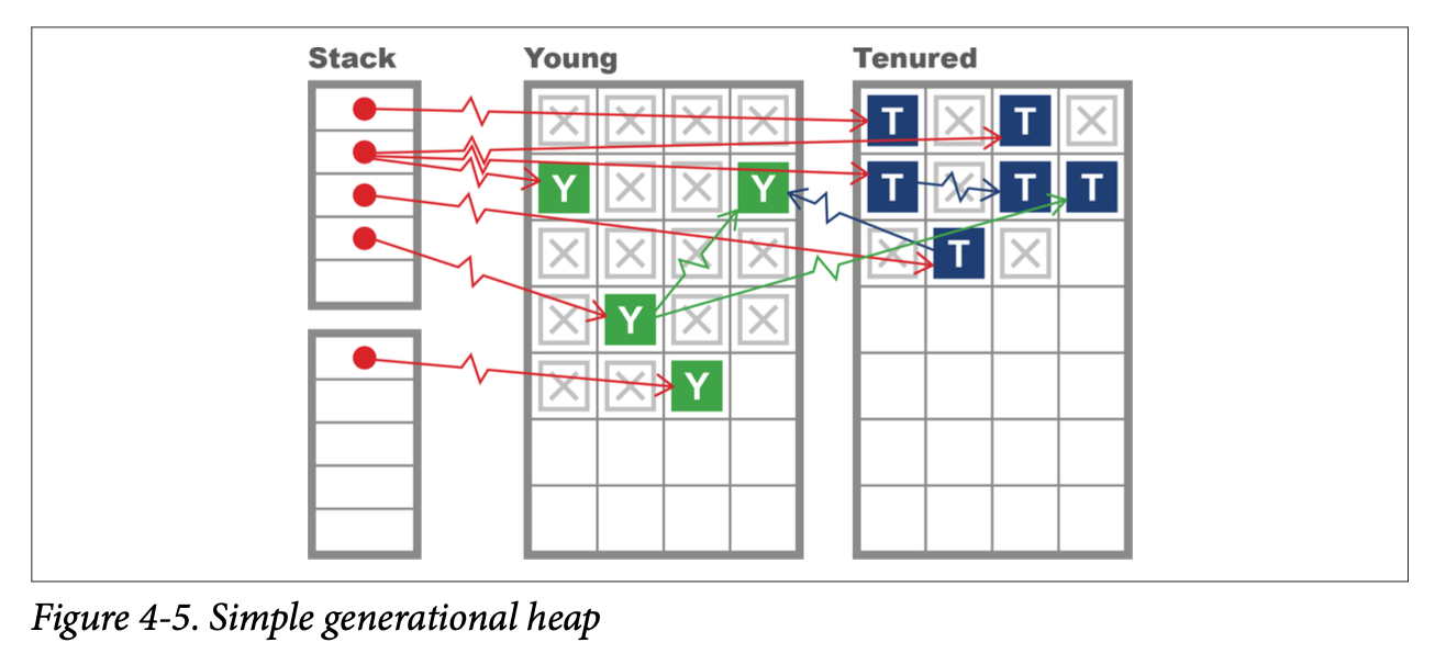
Note that one of the main consequences of using a generational heap is that it costs nothing at all to collect a dead object—there’s simply no bookkeeping to do for it, as we care only about the live objects.

HotSpot uses several mechanisms to try to take advantage of the weak generational hypothesis and to improve on this picture of a generational heap. We’ll meet some of them as we explore the capabilities of a real collector in the next two sections.

Production GC Techniques in HotSpot

In this section, we will build on the theory we’ve met so far and introduce some techniques that will allow us, in the next section, to understand how the simplest production GCs in HotSpot work. Let’s start with one of the most important techniques used to improve allocation performance.

Thread-Local Allocation

Eden is the region of the heap where most objects are created, and very short-lived objects (those with lifetimes less than the remaining time to the next GC cycle) will never be located anywhere else. For this reason, it is a critical region to manage efficiently, because if the WGH holds, then a great many of our objects can be collected at zero cost.

For improved allocation efficiency, HotSpot partitions Eden into buffers and hands out individual regions of Eden for application threads to use as allocation regions for new objects. The advantage of this approach is that each thread knows that it does not have to consider the possibility that other threads are allocating within that buffer. These regions are called thread-local allocation buffers (TLABs).

The exclusive control that an application thread has over its TLABs means that allocation is O(1) for JVM threads. This is because when a thread creates a new object, storage is allocated for the object, and the thread-local pointer is updated to the next free memory address. In terms of C code, this is a simple pointer bump— that is, one additional instruction to move the “next free” pointer onward.

This behavior can be seen in Figure 4-6, where each application thread holds a separate buffer to allocate new objects.

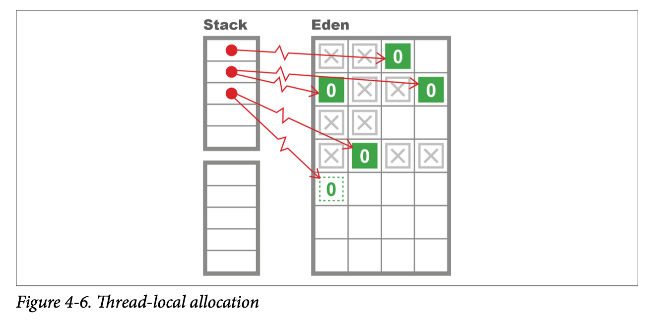
If an application thread fills its current TLAB, then the JVM provides a pointer to a new area of Eden, i.e., a new TLAB. This means that a young GC will occur when the JVM has no more TLABs to hand out.

Hemispheric Collection

One particular special case of the evacuating collector is worth noting. Sometimes referred to as a hemispheric evacuating collector, this type of collector uses two (usually equal-sized) spaces. The central idea is to use the spaces as temporary holding areas for objects that are not actually long-lived. This prevents short-lived objects from cluttering up the tenured generation and reduces the frequency of full GCs.

The spaces have a couple of basic properties:

• When the collector is collecting the currently live hemisphere, objects are moved in a compacting fashion to the other hemisphere, and the collected hemisphere is emptied for reuse.
• One-half of the space is kept completely empty at all times.

This approach does, of course, use twice as much memory as can actually be held within the hemispheric part of the collector. This is somewhat wasteful, but it is often a useful technique if the size of the spaces is not excessive. HotSpot uses this hemispheric approach in combination with the Eden space to provide a collector for the young generation.

The hemispheric part of HotSpot’s young heap is referred to as the survivor spaces. As we can see from the view of VisualGC shown in Figure 4-7, the survivor spaces are normally relatively small as compared to Eden, and the role of the survivor spaces swaps with each young generational collection.

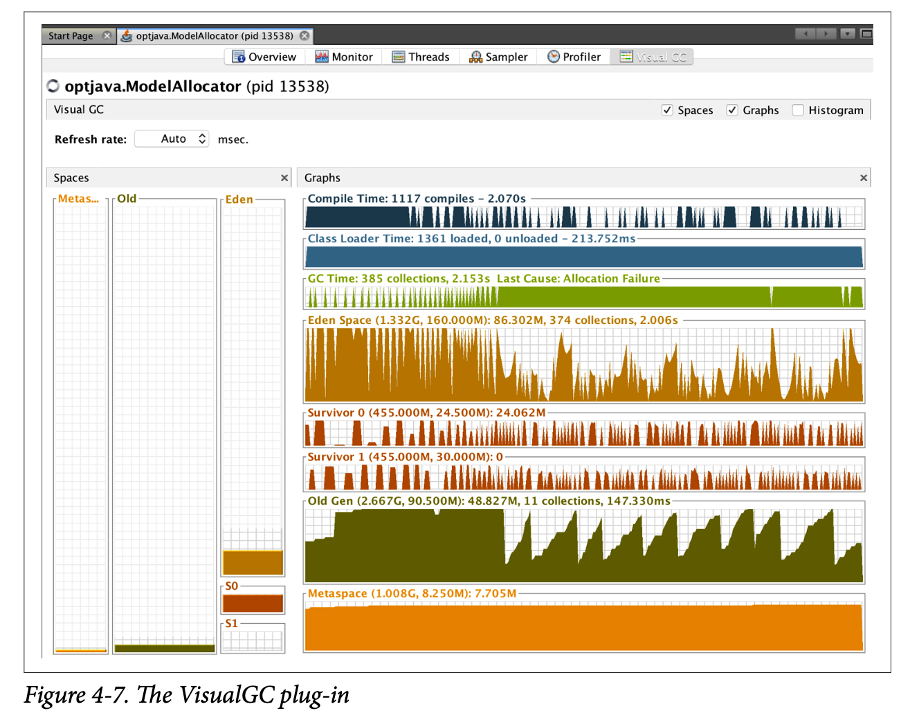
The VisualGC plug-in for VisualVM is a very useful initial GC debugging tool. As we will discuss in Chapter 5, the GC logs contain far more useful information and allow a much deeper analysis of GC than is possible from the moment-to-moment JMX data that VisualGC uses. However, when starting a new analysis, it is often helpful to simply eyeball the application’s memory usage.

Using VisualGC, it is possible to see some aggregate effects of garbage collection, such as objects being relocated in the heap and the cycling between survivor spaces that happens at each young collection.

The “Classic” HotSpot Heap

Let’s bring it all together and describe the basic aspects of the HotSpot heap:

• It tracks the “generational count” of each object (the number of garbage collections that the object has survived so far).
• With the exception of large objects, it creates new objects in the “Eden” space (also called the “nursery”) and expects to move surviving objects to one of two survivor spaces.
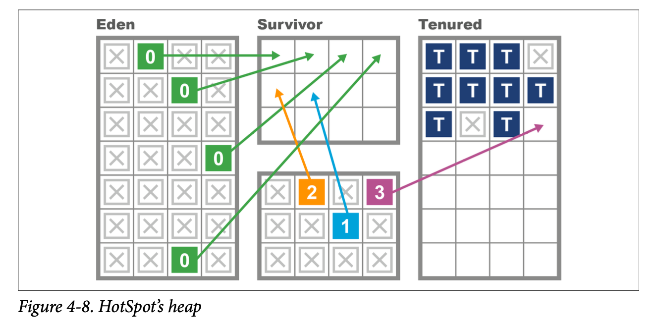
• It maintains a separate area of memory (the “old” or “tenured” generation) to hold objects that are deemed to have survived long enough that they are likely to be long-lived. This approach leads to the view shown in simplified form in Figure 4-8, where objects that have survived a certain number of garbage collection cycles are promoted to the tenured generation. Note the contiguous nature of the regions, as shown in the diagram.

Dividing memory into different regions for purposes of generational collection has some additional consequences in terms of how HotSpot implements a mark-and- sweep collection. One important technique involves keeping track of pointers that point into the young generation from outside. This saves the GC cycle from having to traverse the entire object graph to determine the young objects that are still live.

info

“There are relatively few references from old to young objects” is sometimes cited as a secondary part of the weak generational hypothesis.

To facilitate this process, HotSpot maintains a structure called a card table to help record which old-generation objects could potentially point at young objects. The card table is essentially an array of bytes managed by the JVM. Each element of the array corresponds to a 512-byte area of old-generation space.

info

Later on, we’ll meet remembered sets, which are a more sophistica‐ ted version of the card table.

The central idea is that when a field of reference type on an old object, o, is modified, the card table entry for the card containing the oop corresponding to o is marked as dirty. HotSpot achieves this with a simple write barrier when updating reference fields. It essentially boils down to this bit of code being executed after the field store:

cards[*oop >> 9] = 0;

Note that the dirty value for the card is 0, and the right-shift by 9 bits gives the size of the card table as 512 bytes.

Finally, we should note that this description of the heap in terms of contiguous young and old areas is a historic one—this is the way that Java’s collectors have traditionally managed memory. Modern collectors, such as G1, do not require contiguous storage of the generations—instead, they have regions that still belong to generations but do not need to be colocated with each other.

We will have much more to say about these regional collectors, as we will see in “G1” module. For now, the classic view of the HotSpot heap provides an excellent way to move beyond the simplest, most basic view of tracing garbage collection, and a first step to understanding the realities of production collectors.

Recall that unlike C/C++ and similar environments, Java does not use the operating system to manage dynamic memory. Instead, the JVM allocates (or reserves) memory up front, when the JVM process starts, and manages a single, contiguous memory pool from user space.

As we have seen, this pool of memory is made up of different regions with dedicated purposes, and the address that an object resides at will very often change over time as the collector relocates objects, which are normally created in Eden. Collectors that perform relocation are known as “evacuating” collectors, as mentioned in “Garbage Collection Glossary” module.

Many, but not all, of the collectors that HotSpot ships with are evacuating—let’s meet some simple examples in the next section.

The Parallel Collectors

In Java 8 and earlier versions, the default collectors for the JVM are the parallel collectors. These are fully STW for both young and full collections, and they are optimized for throughput. After stopping all application threads, the parallel collectors use all available CPU cores to collect memory as quickly as possible.

The available parallel collectors are:

Parallel GC — The simplest collector for the young generation

ParNew — A slight variation of Parallel GC that is used with the deprecated Concurrent Mark Sweep collector

ParallelOld— The parallel collector for the old (aka tenured) generation

The parallel collectors are, in some ways, similar to each other—they are designed to use multiple threads to identify live objects as quickly as possible and to do minimal bookkeeping.

info

From Java 17 onward, the Concurrent Mark Sweep (CMS) collector has been removed, and there is only one parallel GC, with the young and old parallel collections being what make up the Parallel GC.

There are some differences between the different collections, so let’s take a closer look.

Young Parallel Collections

The most common type of collection is a young generational collection. This usually occurs when a thread tries to allocate an object into Eden but doesn’t have enough space in its TLAB, and the JVM can’t allocate a fresh TLAB for the thread. When this occurs, the JVM has no choice other than to stop all the application threads—because if one thread is unable to allocate, then very soon every thread will be unable.

info

Threads can also allocate outside of TLABs (e.g., for large blocks of memory). The desired case is when the rate of non-TLAB allocation is low, for several reasons, e.g., too many allocations of short-lived large objects will force additional full GCs, which are more expensive than young collections.

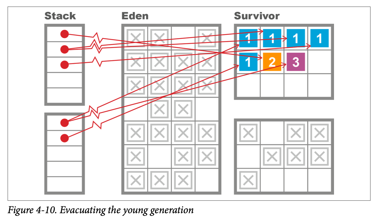
Once all application threads are stopped, HotSpot looks at the young generation (which is defined as Eden and the currently nonempty survivor space) and identifies all objects that are not garbage. This will utilize the GC roots (and the card table to identify GC roots coming from the old generation) as starting points for a parallel marking scan.

The Parallel GC collector then evacuates all of the surviving objects into the currently empty survivor space (and increments their generational count as they are relocated). Finally, Eden and the just-evacuated survivor space are marked as empty, reusable space, and the application threads are started so the process of handing out TLABs to application threads can begin again. This process is shown in Figures 4-9 and 4-10.

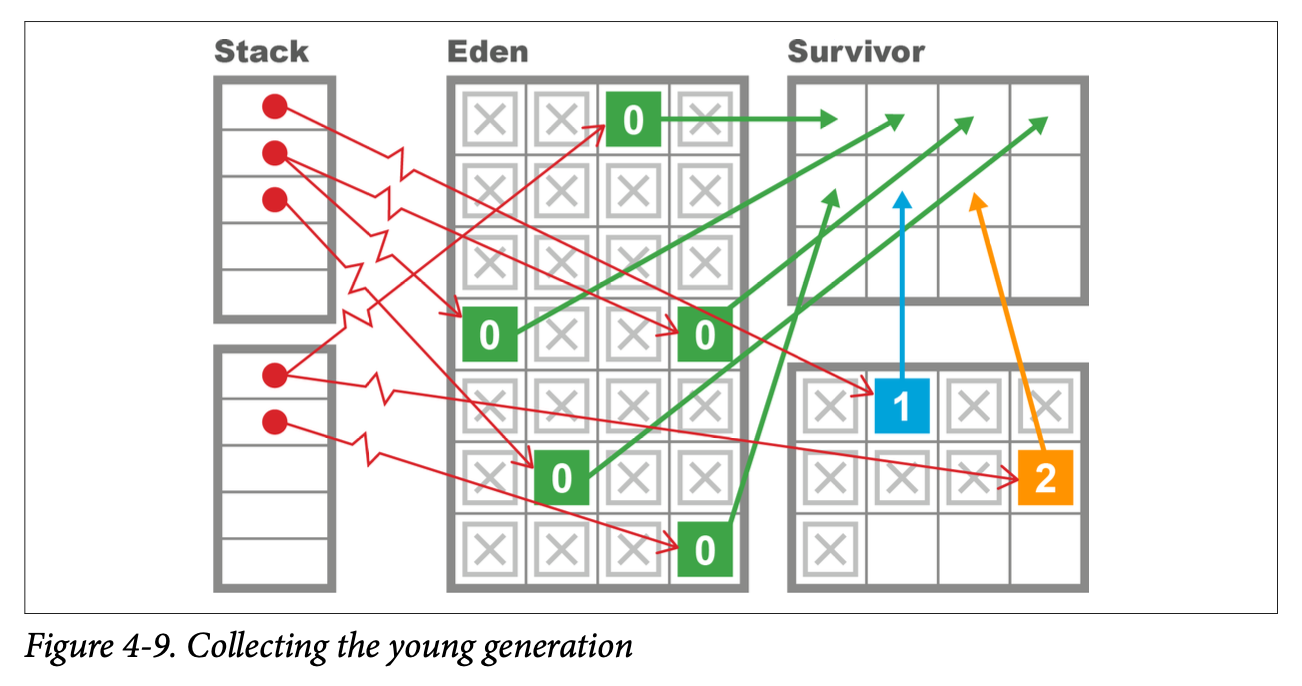
This approach attempts to take full advantage of the weak generational hypothesis by touching only live objects. It also wants to be as efficient as possible and run using all cores as much as possible to shorten the STW pause time.

Old Parallel Collections

The ParallelOld collector was the default collector for the old generation up until Java 8, and for some applications that care primarily about sustained throughput performance, it can still outperform G1

info

As we’ll see in the next chapter, the default for Java 11+ is the G1 collector.

warning

This is especially true for Java 8 applications but less so for Java 11, and by Java 17 it is very difficult to find any workload where Parallel outperforms G1. You have to measure your performance before changing GC algorithm.

It has some strong similarities to Parallel GC but also some fundamental differences. In particular, Parallel GC is a hemispheric evacuating collector, whereas ParallelOld is a compacting collector with only a single continuous memory space.

This means that as the old generation has no other space to be evacuated to, the parallel collector attempts to relocate objects within the old generation to reclaim space that may have been left by old objects dying. Thus, the collector can potentially be very efficient in its use of memory, and it will not suffer from memory fragmentation.

This results in a very efficient memory layout at the cost of using a potentially large amount of CPU during full GC cycles. We saw the evacuating approach in Figures 9 and 10, and the difference between this approach and in-place compaction can be seen in Figure 4-11.

The behavior of the two memory spaces is radically different, as they are serving different purposes. The purpose of the young collections is to deal with the short-lived objects, so the occupancy of the young space is changing radically with allocation and clearance at GC events.

By contrast, the old space does not change as obviously. Occasional large objects will be created directly in tenured, but apart from that, the space will only change at collections—either by objects being promoted from the young generation, or by a full rescan and rearrangement at an old or full collection.

Serial and SerialOld

The Serial and SerialOld collectors are included in this section largely as a cautionary tale.

They operate similarly to the Parallel GC and ParallelOld collectors, but with one important difference—they use only a single CPU core to perform GC. To be absolutely explicit about this—they are not concurrent collectors and are still fully STW.

On multicore systems, the use of these collectors is obviously wrong—as all but one of the CPUs sits idle while a single core performs STW GC. This leads to vastly increased pause times for no benefit, so these collectors should not be used without a conscious choice (see “Containers and GC” on page 232 for an important subtlety).

Limitations of Parallel Collectors

The parallel collectors deal with the entire contents of a generation at once and try to collect as efficiently as possible. However, this design has some drawbacks. First, they are fully stop-the-world. This is not usually an issue for young collections, as the weak generational hypothesis means that very few objects should survive.

info

The design of the young parallel collectors is such that dead objects are never touched, so the length of the marking phase is proportional to the (small) number of surviving objects.

This basic design, coupled with the usually small size of the young regions of the heap, means that the pause time of young collections is very short for most workloads. A typical pause time for a young collection on a modern 2 GB JVM ( with default sizing) might well be just a few milliseconds—and may even by submillisecond.

However, collecting the old generation is often a very different story. For one thing, the old generation is by default seven times the size of the young generation. This fact alone will make the expected STW length of a full collection much longer than for a young collection.

Another key fact is that the marking time is proportional to the number of live objects in a region. Old objects may be long-lived, so a potentially larger number of old objects may survive a full collection.

This behavior also explains a key weakness of ParallelOld collection--the STW time will scale roughly linearly with the size of the heap. As heap sizes continue to increase, ParallelOld starts to scale badly in terms of pause time.

Newcomers to GC theory sometimes entertain private theories that minor modifications to mark-and-sweep algorithms might help to alleviate STW pauses. However, this is not the case.

Garbage collection has been a very well-studied research area of computer science for over 40 years, and production collectors are complex, with many tradeoffs. It is extremely unlikely that any such “can’t you just...” tweak will yield any generally applicable improvement.

As we will see in Chapter 5, mostly concurrent collectors do exist, and they can run with greatly reduced pause times. However, they are not a panacea, and several fundamental difficulties with garbage collection remain.

As an example, let’s consider TLAB allocation. This provides a great boost to allocation performance but is of no help to collection cycles. To see why, consider this code:

public static void main(String[] args) {
    int[] anInt = new int[1];
    anInt[0] = 42;
    Runnable r = () -> {
        anInt[0]++;
        System.out.println("Changed: " + anInt[0]);
    };
    new Thread(r).start();
}

The variable anInt is an array object containing a single int. It is allocated from a TLAB held by the main thread but immediately afterward is passed to a new thread. To put it another way, the key property of TLABs—that they are private to a single thread—is true only at the point of allocation. This property can be violated as soon as objects have been allocated.

The Java environment’s ability to trivially create new threads is a fundamental, and extremely powerful, part of the platform. However, it complicates the picture for garbage collection considerably, as new threads imply execution stacks, each frame of which is a source of GC roots.

The Role of Allocation

Java’s garbage collection process is most commonly triggered when memory allocation is requested but there is not enough free memory on hand to provide the required amount. This means that GC cycles do not occur on a fixed or predictable schedule but purely on an as-needed basis.

This is one of the most critical aspects of garbage collection: it is not deterministic and does not occur at a regular cadence. Instead, a GC cycle is triggered when one or more of the heap’s memory spaces are essentially full, and further object creation would not be possible. This means, in the language of Chapter 10, that GC behavior is represented as events, and needs to be aggregated to produce metrics.

warning

Some Java GCs have ways to configure periodic GCs, which are time-based—do a GC at least every N (milli)seconds if not otherwise triggered. This feature may appear superficially attractive, but in practice it is rarely useful and can be a source of performance problems as developers try to “outhink the GC.”

tip

The as-needed nature of GC events makes them hard to process using traditional time series analysis methods. The lack of regularity between GC events is an aspect that most time series libraries cannot easily accommodate.

When an STW GC occurs, all application threads are paused (as they cannot create any more objects, and no substantial piece of Java code can run for very long without producing new objects). The JVM takes over all of the cores to perform GC and reclaims memory before restarting the application threads.

To better understand why allocation is so critical, let’s consider the following highly simplified case study. The heap parameters are set up as shown, and we assume that they do not change over time. Of course, a real application would normally have a dynamically resizing heap, but this example serves as a simple illustration:

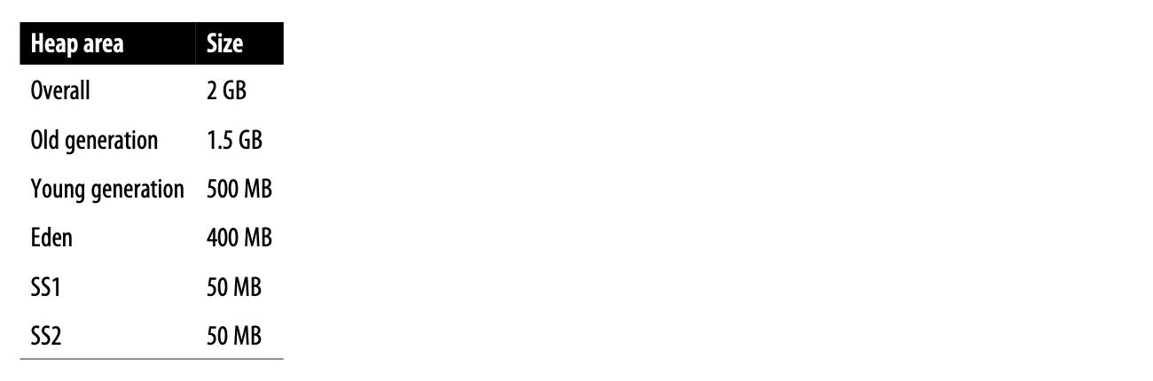
After the application has reached its steady state, the following GC metrics are observed:

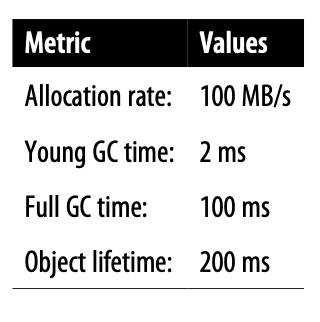
This shows that Eden will fill in 4 seconds, so at steady state, a young GC will occur every 4 seconds. Eden has filled, so GC is triggered. Most of the objects in Eden are dead, but any object that is still alive will be evacuated to a survivor space (S1, for the sake of discussion). In this simple model, any objects that were created in the last 200 ms have not had time to die, so they will survive. So, we have:

GC0 @4s 20MBEden→SS1(20MB)

After another 4 seconds, Eden refills and will need to be evacuated (to SS2 this time). However, in this simplified model, no objects that were promoted into SS1 by GC0 survive—their lifetime is only 200 ms, and another 4 s has elapsed, so all of the objects allocated prior to GC0 are now dead. We now have:

GC1 @8.002s 20MBEden→SS2(20MB)

Another way of saying this is that after GC1, the contents of SS2 consist solely of objects newly arrived from Eden, and no object in SS2 has a generational age > 1. Continuing for one more collection, the pattern should become clear:

GC2 @12.004s 20MBEden→SS1(20MB)

This idealized, simple model leads to a situation where no objects ever become eligible for promotion to the old generation, and the space remains empty throughout the run. This is, of course, very unrealistic.

Instead, the weak generational hypothesis indicates that object lifetimes will be a distribution, and due to the uncertainty of this distribution, some objects will end up surviving to reach tenured.

Let’s look at a very simple simulator for this allocation scenario. It allocates objects, most of which are very short-lived but some of which have a considerably longer life span. It has a couple of parameters that define the allocation: x and y, which between them, define the size of each object; the allocation rate (mbPerSec); the lifetime of a short-lived object (shortLivedMS) and the number of threads that the application should simulate (nThreads). The default values are here:

(Omitting main() and any other startup/parameter-setting code)

public class ModelAllocator implements Runnable {
    private volatile boolean shutdown = false;
    private double chanceOfLongLived = 0.02;
    private int multiplierForLongLived = 20;
    private int x = 1024;
    private int y = 1024;
    private int mbPerSec = 50;
    private int shortLivedMs = 100;
    private int nThreads = 8;
    private Executor exec = Executors.newFixedThreadPool(nThreads);

    public void run() {
        final int mainSleep = (int) (1000.0 / mbPerSec);
        while (!shutdown) {
            for (int i = 0; i < mbPerSec; i++) {
                ModelObjectAllocation to =
                        new ModelObjectAllocation(x, y, lifetime());
                exec.execute(to);
                try {
                    Thread.sleep(mainSleep);
                } catch (InterruptedException ex) {
                    shutdown = true;
                }
            }
        }
    }

    // Simple function to model weak generational hypothesis
    // Returns the expected lifetime of an object - usually this // is very short, but there is a small chance of an object // being "long-lived"
    public int lifetime() {
        if (Math.random() < chanceOfLongLived) {
            return multiplierForLongLived * shortLivedMs;
        }
        return shortLivedMs;
    }
}

The allocator main runner is combined with a simple mock object used to represent the object allocation performed by the application:

public class ModelObjectAllocation implements Runnable {
    private final int[][] allocated;
    private final int lifeTime;

    public ModelObjectAllocation(final int x, final int y, final int liveFor) {
        allocated = new int[x][y];
        lifeTime = liveFor;
    }

    @Override
    public void run() {
        try {
            Thread.sleep(lifeTime);
            System.err.println(System.currentTimeMillis() + ": "
                    + allocated.length);
        } catch (InterruptedException ex) {
        }
    }
}

When seen in VisualVM, this will display the simple sawtooth pattern often observed in the memory behavior of Java applications that are making efficient use of the heap. This pattern can be seen in Figure 4-12.

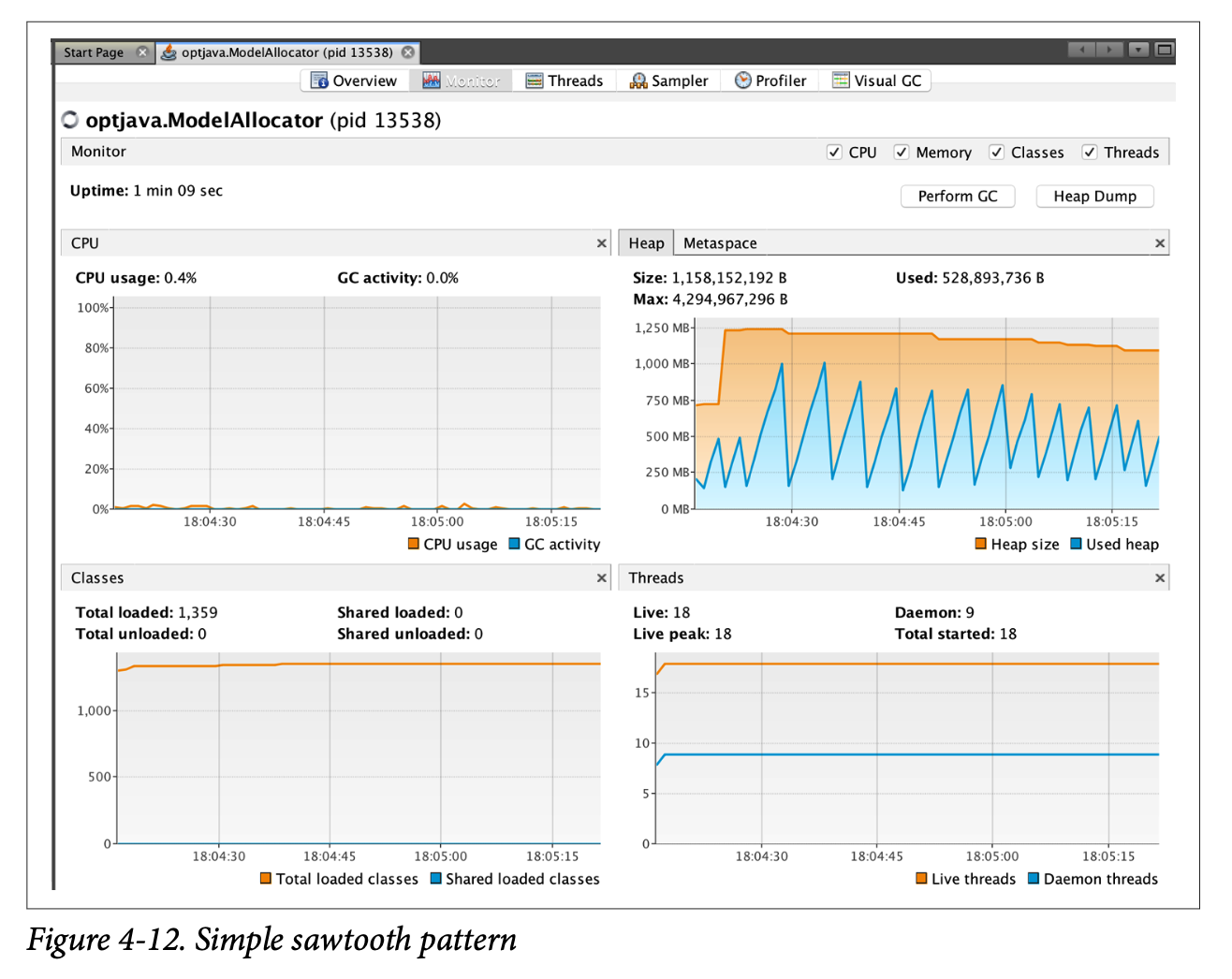
The interested reader can download the allocation and lifetime simulator referenced in this chapter and set parameters to see the effects of allocation rates and percentages of long-lived objects.

info

Amazon provides its HyperAlloc tool, part of the Heapothesys project. This benchmarking tool is “a synthetic workload which simulates fundamental application characteristics that affect garbage collector latency.”

To finish this discussion of allocation, we want to shift focus to a very common aspect of allocation behavior. In the real world, allocation rates can be highly changeable and “bursty.” Consider the following scenario for an application with a steady-state behavior as previously described:

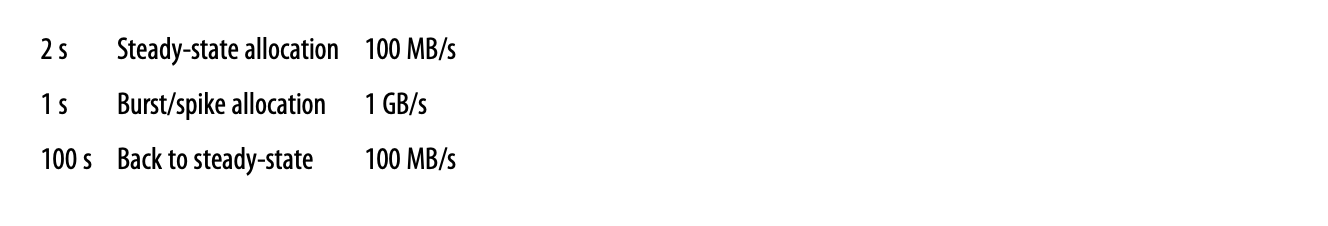
The initial steady-state execution has allocated 200 MB in Eden. In the absence of long-lived objects, all of this memory has a lifetime of 100 ms. Next, the allocation spike kicks in. This allocates the other 200 MB of Eden space in just 200 ms, and of this, 100 MB is under the 100 ms age threshold. The size of the surviving cohort is larger than the survivor space, so the JVM has no option but to promote these objects directly into tenured. So we have:

GC0 @ 2.2 s 100 MB Eden → Tenured (100 MB)`

The sharp increase in allocation rate has produced 100 MB of surviving objects, although note that in this model all of the “survivors” are, in fact, short-lived and will very quickly become dead objects cluttering up the tenured generation. They will not be reclaimed until a full collection occurs.

Continuing for a few more collections, the pattern becomes clear:

GC1 @ 2.602 s   200 MB Eden → Tenured (300 MB)
GC2 @ 3.004 s   200 MB Eden → Tenured (500 MB)
GC3 @ 7.006 s   20 MB Eden → SS1 (20 MB) [+ Tenured (500 MB)]

Notice that, as discussed, the garbage collector runs as needed, and not at regular intervals. The bigger the allocation rate, the more frequent are GCs. If the allocation rate is too high, then objects will end up being forced to be promoted early.

This phenomenon is called premature promotion; it is one of the most important indirect effects of garbage collection and a starting point for many tuning exercises, as we will see in the next chapter.

Summary

The subject of garbage collection has been a lively topic of discussion within the Java community since the platform’s inception. In this chapter, we have introduced the key concepts that performance engineers need to understand to work effectively with the JVM’s GC subsystem:

• Mark-and-sweep collection
• HotSpot’s internal runtime representation for objects
• The weak generational hypothesis
• Practicalities of HotSpot’s memory subsystems
• The parallel and serial collectors
• Allocation and the central role it plays

In the next chapter, we will discuss topics in modern GC—including concurrent collectors and HotSpot’s default collector (G1) as well as less-common alternatives, such as Shenandoah and ZGC.

Several of the concepts we met in this chapter—especially allocation and specific effects such as premature promotion—will be of particular significance to the upcoming chapter, and it may be helpful to refer back to this material frequently.